Physics of Low Temperature Plasmas via Particle Simulation

J.P. Boeuf

LAPLACE (Laboratoire Plasma et Conversion d’Energie), Université de Toulouse, CNRS, INPT, UPS
118 route de Narbonne, 31062 Toulouse, France
jpboeuf@laplace.univ-tlse.fr — jpboeuf@gmail.com — jpboeuf.fr

About this document. This document is the printable companion of the test-case library of JC-PIC, a one-dimensional (1D3V) Particle-In-Cell / Monte-Carlo-collisions code for low-temperature plasmas. JC-PIC was written with two aims: to gather and revisit in one place, through simulations that reproduce published results, the main physics that kinetic simulations have taught us over the last decades, and to make kinetic plasma simulation accessible to non-specialists — students, teachers and researchers — through a fully graphical interface that requires no programming. The code, its manual and the case library have been freely available at jc-pic.org since September 2026; each case of this document can be downloaded there, run and modified. The cases are organised by topic; each gives its physical background, the exact simulation conditions, the results with commented figures, and the references. The text and figures below are those of the case files distributed with the code; this version was generated on 07 September 2026. Persistent identifier of this document: doi:10.5281/zenodo.22258142.

Abstract

Particle-In-Cell simulations with Monte-Carlo collisions (PIC-MCC) have, over the last two decades, become a central tool for understanding the physics of low-temperature plasmas: electron power absorption in capacitively and inductively coupled discharges, instabilities in the magnetized plasmas of electric thrusters and magnetrons, the influence of secondary electron emission on wall sheaths and plasma potential, pattern formation and striations in plasma columns, and many other phenomena central to practical applications are now far better understood thanks to these kinetic models. JC-PIC is a one-dimensional (1D3V) PIC-MCC code built around this body of work with a two-fold purpose: to gather and revisit, in one place, the main conclusions of these studies — reproducing the results of a number of published papers, here in one dimension — and to make kinetic plasma simulation genuinely accessible, through a fully graphical, code-free interface usable for research as well as for teaching. This document presents the bundled test-case library: a set of ready-to-run cases, organized by topic (basic plasma physics, electron emission and diodes, DC and transient glow discharges, capacitive RF discharges, positive columns, magnetized plasmas and kinetic instabilities), each reproducing and commenting a published PIC-MCC result under conditions identical or close to the original, with the corresponding references, and each runnable by a non-expert on an ordinary desktop computer.

I Introduction

In the Particle-In-Cell (PIC) method a plasma is represented by a large number of charged super-particles moving in phase space under the self-consistent electromagnetic field computed, at each time step, on a fixed spatial mesh. Combined with a Monte-Carlo treatment of the collisions between charged particles and the neutral gas (PIC-MCC), it is a kinetic method: it follows the evolution of the charged-particle distribution functions and is, in effect, equivalent to solving the Boltzmann equations coupled to Poisson's equation in the electrostatic case. These particle-mesh methods, developed since the 1960s and described in the classic texts of Birdsall & Langdon and of Hockney & Eastwood, were adopted by the low-temperature-plasma community at the end of the 1980s with the addition of the Monte-Carlo collision module.

Over the last two decades PIC-MCC simulations have clarified a wide range of phenomena central to gaseous electronics and plasma processing — electron power absorption (the “stochastic” or collisionless heating) in capacitive and inductive discharges, instabilities in the magnetized plasmas of Hall thrusters and magnetrons, the role of secondary electron emission at the walls, striations and pattern formation in plasma columns, and many others. Where early simulations could follow only a few thousand particles, an ordinary desktop now handles several million, so that one-dimensional kinetic studies of these devices have become routine — yet, in practice, setting up a research-grade PIC-MCC code and extracting meaningful diagnostics from it still demands considerable programming effort, which keeps the method the preserve of specialists.

JC-PIC was written to remove that barrier. It is a one-dimensional, three-velocity-component (1D3V) electrostatic PIC-MCC code — a single spatial coordinate across a plasma column or between two parallel electrodes, with the three velocity components of every super-particle retained so that magnetic fields and the full angular distribution of collisions are handled correctly. The numerical scheme it implements is entirely standard and shared with many other codes; what is unusual is the complete graphical environment built around it, which lets a non-expert load the conditions of a published simulation (gas, pressure, dimensions, wall interaction, voltage waveform or periodic boundaries), run it — most cases on a desktop computer — and inspect the results (density profiles, electron energy distributions, ion flux-energy distributions at the walls, position–time diagrams and more) without writing a single line of code.

The project pursues two complementary aims. The first is pedagogical and exploratory: to place a genuine kinetic simulation in the hands of experimentalists, students and teachers, so that the key results of the modern PIC-MCC literature can be reproduced, examined and understood at first hand. The second is scientific: to revisit the physics of low-temperature discharges in the light of those simulations, gathering and summarizing in one place the main conclusions of a large body of published work. The aim is not to add yet another review, but to select some of the most striking properties of these plasmas and to illustrate and comment on them through simulations carried out under conditions identical or close to those of the original papers.

This document collects the test-case library that ships with JC-PIC and embodies both aims. Each case is a ready-to-run configuration that reproduces a published result, accompanied by a short account of the physics, the simulation conditions, and a discussion of the results, with references to the original papers. The library is organized by topic, following the structure of the sections below: fundamentals of plasma physics (sheaths, diffusion, waves, expansion); electron emission from cathodes and space-charge-limited diodes; DC and transient glow discharges, including plasma-immersion ion implantation; capacitively coupled radio-frequency discharges (benchmarks, electron heating, electrical and magnetic asymmetry, frequency effects); the positive column and its striations; magnetized plasmas; and the classic kinetic beam instabilities. Together they form both a hands-on tutorial in kinetic simulation and a compact, illustrated review of low-temperature plasma physics as seen through particle simulations.

II Basic Plasma Physics

This chapter is the pedagogical core of the library. It is a set of small, fully controlled simulations. In these simulations the classical results of plasma physics can be checked number by number. The effects that fluid theory cannot describe can be seen directly in the particle data: wave-particle interaction, trapping in phase space, and the loss of quasineutrality at a wall.

This chapter assumes the elementary material and does not develop it. A reader who wants the definitions first will find them in the Appendix at the end of the library. These definitions are the Debye length, the plasma and cyclotron frequencies, the thermal speeds and the distributions, and the way they determine the cell size and the time step of a simulation. The Appendix also contains two interactive sections that are outside the progression. Single-Particle Motion shows how one charged particle moves in imposed fields. Collisions and Cross Sections opens the cross-section data on which every case here depends. Neither needs a run; both answer in milliseconds.

A note on units. In the whole library, electron and ion temperatures are given in electron-volts, as is usual in plasma physics (1 eV = 11 605 K). Tₑ = 2 eV means that the thermal energy kB Tₑ is 2 eV. The formulas are written with this convention: the Bohm speed is √(eTₑ/M), a Boltzmann factor is exp(Φ/Tₑ), and a potential drop written Tₑ/2 or 4 Tₑ is in volts. Gas and cathode temperatures, on the contrary, are given in kelvin (a gas density is p/kB Tg).

The sections follow a simple progression.

The first question is what happens where a plasma meets a wall. In Plasma Sheath - Plasma Potential, the plasma potential forms by itself, the ions reach the Bohm velocity, and collisions then redistribute the potential between the sheath and the bulk.

When a magnetic field meets the wall at an angle, a second layer forms in front of the Debye sheath. The Sheath in an Oblique Magnetic Field section follows the ion flow through this layer. The ions are first accelerated along the magnetic field, then turned towards the wall over a distance of the order of their Larmor radius. Two conditions have to be satisfied one after the other: the Chodura condition along the field, and the Bohm condition at the entrance of the Debye sheath.

Collisional Plasma Diffusion and Plasma Expansion treat transport. The first is the ambipolar field that forces electrons and ions to diffuse together through a gas. The second, at the opposite extreme, is the free expansion of a plasma into vacuum with its supersonic ion front.

Two sections are about waves. Langmuir Waves isolates the fast electron oscillations, from the linear Bohm-Gross dispersion to non-linear electron trapping. Ion Acoustic Waves treats the slow, ion-scale waves, with the kinetic effects that come with them: Landau damping and wave breaking.

Finally, PIC-MCC and Global Model compares the spatially resolved kinetic simulation with the zero-dimensional global models commonly used for reactor design. It shows what a global model gets right, and what it cannot know.

II.A Plasma Sheath & Plasma Potential: Fundamental Principles

A plasma cannot be in contact with a wall without being perturbed. Electrons are thousands of times lighter than ions, so they reach any surface much faster. A wall in contact with a plasma therefore charges negatively, until the electric field that it has created holds the electrons back. This field is located in a thin positive layer along the wall, the sheath, which is a few Debye lengths thick. In this layer quasineutrality is broken. The field slows the electrons down and accelerates the ions. As a result, the bulk of the plasma is at a positive potential with respect to the wall. This potential is the plasma potential. Its value adjusts itself until electrons and ions are lost at exactly the same rate.

Sheath and presheath

The transition from the plasma to the wall has two parts. The sheath can exist only if the ions enter it fast enough, that is at least at the ion sound speed $c_s = \sqrt{e T_e / M}$. This is the Bohm criterion. The ions are accelerated to this speed in a wider quasineutral region in front of the sheath, the presheath. The presheath carries a small potential drop, about $T_e/2$ in the simplest model. The total drop from the plasma to the wall is therefore the sum of two terms. The large sheath part is fixed by the balance of the electron and ion fluxes. The small presheath part is fixed by the Bohm criterion. For helium the sum given in textbooks is close to $4\,T_e$.

How these cases are built

The three cases of this section keep only the sheath physics and remove everything else. There is no real ionization. Electron-ion pairs are injected by an imposed volumetric source at a fixed rate, so the wall flux is known in advance. The electron temperature is held at 2 eV by a simple thermostat, so all the quantities that depend on $T_e$ are controlled. In these simple conditions the potential profile, the presheath drop and the ion velocities can be compared with the theory, number by number.

• Uniform Collisionless Plasma Source — the standard case: the source is everywhere and there are no collisions. The Bohm criterion is verified at the sheath entrance. The measured plasma potential is 8.0 V, which agrees to 2 % with the analytical $4\,T_e$ estimate.

• Limited Collisionless Plasma Source — the same plasma, but the source is limited to the central fifth of the gap. The ions now reach the sound speed at the exit of the source region, far from the walls, and the plasma potential decreases to $3\,T_e$ at the same electron temperature. This case shows that the potential is fixed by a flux balance, and not by $T_e$ alone. In a collisionless plasma it depends on the way the tail of the electron distribution is refilled.

• Influence of Collisions — the same plasma again, at 0, 10, 40 and 100 mTorr. Ion-neutral collisions confine the plasma: the central density increases by a factor 4.3 for the same source. They also move the potential drop out of the sheath and into the bulk, and the part of the drop inside the plasma increases from one fifth to four fifths. In the collisionless case the ions arrived at the wall with the full potential drop. Here they arrive with a broad energy distribution, at lower energies.

II.A. Case 1 Uniform, Collisionless Plasma Source

In this test case a collisionless plasma is generated by a spatially uniform external source of electrons and ions between two grounded electrodes. The source creates electron-ion pairs with Maxwellian distributions at temperatures $T_e$ and $T_i$. Electrons are lost to the grounded electrodes much faster than ions. Therefore two space-charge sheaths form next to the electrodes, where an electric field limits the flux of electrons to the walls. As a result, the plasma potential increases with respect to the potential of the wall electrodes. Intuitively, the plasma potential is larger for larger electron temperatures. The discussion below applies to a plasma between grounded electrodes, but also to a plasma contained by dielectric walls.

In a real plasma source, the electron temperature is maintained by various electron heating methods. Examples are the injection of electrons from a filament at a negative potential with respect to the plasma, inductive radiofrequency coupling, etc. To keep the simulation simple and to concentrate on the formation and properties of the sheath, an idealized form of electron heating must be applied. If electron heating is not implemented in the simulation, the fast electrons of the Maxwellian source are quickly lost to the walls. This leads to a continuous decrease of the electron temperature and of the plasma potential. Therefore a simulation with a plasma source but without electron heating cannot maintain the electron temperature. It does not lead to a realistic steady state (what would be the electron temperature at steady state?). Recent PIC-MCC simulations of sheath formation with a uniform plasma source [1], [2] are run in exactly this configuration, without electron heating, and report steady-state sheaths at low pressure. The question above has no answer. Without collisions to repopulate the escape region of velocity space, an electron created below the potential barrier is trapped permanently. The trapped population accumulates without limit, and the electron temperature has no value to converge to. It cannot converge to the source temperature, and it cannot converge to the gas temperature, because at these pressures there are no electron-neutral collisions to thermalise with. A steady state can only be sustained by a process that repopulates the barrier. This process can be real collisions, real heating, or numerical heating from the grid and from a limited number of macroparticles per cell. JC-PIC does not reproduce these results, and it should not.

In the simulation presented here, the electron heating is done as follows. Each time an electron crosses the mid-gap plane, it is reinjected in the same direction. Its speed is resampled from a half-Maxwellian flux distribution with a thermal spread determined by the source temperature. In these collisionless conditions this method ensures a perfectly uniform electron temperature in the quasineutral plasma. This “refluxing” process has been used to study the plasma-sheath region in the group of C. K. Birdsall, and is described in Procassini et al. [3].

Physics

The plasma-wall transition has a well-known two-scale structure [4]-[5]. There is a quasineutral region including a presheath, where a weak electric field pre-accelerates the ions toward the walls. There is also a thin, positively charged sheath (a few electron Debye lengths $\lambda_{De}$ thick) next to each electrode, which confines most of the electrons electrostatically. The plasma potential at steady state adjusts itself so that electrons and ions are lost at exactly the same rate. Its value can be derived in three steps.

Bohm criterion The sheath is a region of positive space charge: the ion density must be larger than the electron density everywhere inside it. This is possible only if the ions enter the sheath fast enough [6], [7]. Let $V(x)<0$ be the potential relative to the sheath edge, and $u_s$ the directed ion velocity at the sheath edge. The cold ions cross the collisionless sheath with conservation of their energy ($Mu^2/2 = Mu_s^2/2 - eV$) and of their flux ($n_i u = n_s u_s$). The electron density follows the Boltzmann relation ($T_e$ in eV):

Both densities are expanded to first order in the small potential $|V|$ just inside the sheath. This gives the space charge $n_i - n_e \simeq n_s V \left(e/Mu_s^2 - 1/T_e\right)$. Since $V<0$, the space charge is positive only if:

where $M$ is the ion mass. This is the Bohm criterion. A stationary, monotonic sheath can only form if the ions enter it at least at the Bohm velocity $u_B$ (in practice the criterion is marginally satisfied, $u_s \simeq u_B$).

Presheath potential drop In the quasineutral region the electrons are nearly in Boltzmann equilibrium, $n(x) = n_0 \exp\left[\left(\Phi(x)-\Phi_p\right)/T_e\right]$, where $n_0$ and $\Phi_p$ are the density and the plasma potential at the center. In the simple fluid model, ions starting from rest reach the Bohm velocity at the sheath edge. Energy conservation, $Mu_B^2/2 = e\Delta\Phi_{pre}$, then gives the potential drop across the presheath:

and the density at the sheath edge is $n_s = n_0\exp(-1/2) \simeq 0.61 n_0$.

Sheath potential drop In steady state a grounded (or floating) wall must collect equal electron and ion fluxes. The ion flux entering the sheath is the Bohm flux $\Gamma_i = n_s u_B$ (the sheath is collisionless, so this flux reaches the wall). The electron flux is the thermal flux reduced by the Boltzmann factor of the sheath potential drop $\Delta\Phi_{sh}$:

Writing $\Gamma_e = \Gamma_i$ gives:

The plasma potential (with respect to the grounded walls) is the sum of the presheath and sheath drops:

For helium ($M/m = 7296$) this gives $\Delta\Phi_{sh} \simeq 3.5 T_e$ and $\Phi_p \simeq 4.0 T_e$, i.e. $\Phi_p \simeq 8.1$ V for $T_e = 2$ eV. This is in very good agreement with the simulation results below. This value depends on one hidden assumption: the electron distribution must remain Maxwellian up to the escape energy. Here the mid-plane thermostat guarantees this. The Limited Collisionless Plasma Source case shows what happens when this assumption fails: with the same $T_e$, the plasma potential decreases to 3 $T_e$.

Kinetic refinements The fluid estimate above is robust. However, the problem treated here is exactly the “free-fall” regime first solved kinetically by Tonks and Langmuir [4]. In this regime ions are created at rest throughout the volume and fall freely, without collisions, in the self-consistent field. The kinetic solution gives a slightly larger presheath drop ($\simeq 0.85 T_e$ in plane geometry) and a Bohm criterion generalized to an arbitrary ion velocity distribution (marginally satisfied at the sheath edge). The mathematical structure of the plasma-sheath transition in the limit $\lambda_{De}/L \rightarrow 0$ is analyzed in depth in the classical review of Riemann [7]. Textbook derivations can be found in Lieberman and Lichtenberg [5]. Discussions of sheath physics compared with experiments are given by Hershkowitz [8] and in the tutorial review of Robertson [9].

Simulation conditions

• Gas: Helium at $p = 0$ (no collisions; the neutral gas plays no role).
• Domain: 5 cm gap between two grounded, absorbing electrodes.
• Initial conditions: uniform plasma density 10¹⁴ m⁻³, electron and ion temperatures $T_e = 2$ eV and $T_i = 0.026$ eV.
• Plasma source: uniform volumetric source of electron-ion pairs over the whole gap, at a rate equivalent to $J_0 = 0.2$ A/m², with Maxwellian distributions at $T_e = 2$ eV and $T_i = 0.026$ eV.
• Electron heating: refluxing at the mid-gap plane with an electron temperature of 2 eV (see above).
• Numerics: 400 grid cells ($\Delta x = 0.125$ mm, well below $\lambda_{De} \simeq 1$ mm), 80000 particles at the beginning (200 per cell), time step $5\times 10^{-11}$ s.

Results

Figure 1: Profiles of the charged particle densities and of the plasma potential at steady state.

The bulk of the plasma is quasineutral ($n_e \simeq n_i$), with a density maximum of about $1.4\times 10^{14}$ m⁻³ at the center. Although the source is spatially uniform, the density decreases toward the walls. The reason is that the ions are continuously accelerated in the free-fall presheath, so flux conservation requires a decreasing density. The two sheaths are clearly visible near the electrodes, where $n_i > n_e$. The plasma potential has a flat top at $\Phi_p \simeq 8$ V, i.e. $\Phi_p \simeq 4 T_e$. This agrees to 2 % with the analytical estimate of the Physics section: about 1 V ($\simeq T_e/2$) is dropped across the quasineutral presheath and about 7 V ($\simeq 3.5 T_e$) across each sheath.

Figure 2: Profiles of the space charge and of the electric field at steady state.

The space charge $n_i - n_e$ fluctuates around zero in the bulk (PIC statistical noise) and becomes strongly positive in the two sheaths. The thickness of the sheaths, a few mm, corresponds to a few Debye lengths. The electric field is antisymmetric with respect to the mid-gap. It reaches about $2.5\times 10^{3}$ V/m at the electrodes and is very small, but not zero, in the quasineutral region. This weak presheath field is the field that accelerates the ions up to the Bohm velocity at the sheath edges.

Figure 3: Spatial distribution of the parallel, perpendicular and total electron temperatures.

The refluxing thermostat maintains a uniform and isotropic electron temperature of 2 eV over the whole quasineutral plasma ($T_{e\parallel} \simeq T_{e\perp} \simeq T_e$). The small spike at $x = 2.5$ cm is the signature of the refluxing plane. Inside the sheaths the parallel temperature decreases. Only the electrons with enough parallel energy to climb the potential barrier enter the sheaths, and they are decelerated as they climb. The perpendicular velocities are not affected. This is a purely kinetic (non-Maxwellian) boundary effect.

Figure 4: Spatial distribution of the parallel, perpendicular and total ion temperatures.

The perpendicular ion temperature remains at the source value (0.026 eV): without collisions, nothing acts on the perpendicular velocities. The “parallel temperature”, in contrast, increases toward the walls up to $\simeq 0.9$ eV. This is not collisional heating. At a given position, the parallel velocity distribution mixes ions born at different locations, which have therefore fallen through different potential drops. This spread of arrival velocities appears as an effective parallel temperature. It is a kinetic feature characteristic of presheaths with a distributed cold-ion source (ion heating in presheaths is discussed in a different, collisional and unstable context in [2]).

Figure 5: Profile of the mean ion velocity normalized to the Bohm velocity.

The mean ion velocity $\langle v_x \rangle_i$, normalized to the Bohm velocity ($u_B \simeq 6.9$ km/s for helium at $T_e = 2$ eV), increases smoothly from zero at the center. It reaches $u_B$ at the entrance of the sheaths. In other words, the Bohm criterion is marginally satisfied at the sheath edges, as expected from theory [6], [7]. Inside the sheaths the ions become strongly supersonic and hit the electrodes at about $2.4 u_B$.

Figure 6: Ion flux energy distribution at the electrodes.

The energy distribution of the ion flux collected by the electrodes shows a sharp peak at $\varepsilon \simeq 8$ eV $= e\Phi_p$. These are the ions created in the central region, where the potential is flat, which fall through the full potential drop. The low-energy shoulder corresponds to ions created closer to the walls, at a lower local potential. The distribution is sharply cut off above $e\Phi_p$ (the source ions are cold and there are no collisions, so no ion can gain more than the full potential drop). The left and right distributions are identical, as required by the symmetry of the problem.

Figure 7: Power balance at steady state.

The power balance closes to within the statistical noise (residual $\simeq 4\times 10^{-5}$ W/m², five orders of magnitude below the fluxes). This confirms that a true steady state is reached. The energy input is shared between the source ($0.61$ W/m² $= (3/2)(T_e+T_i) J_0/e$, almost entirely carried by the electrons) and the refluxing thermostat ($1.59$ W/m²). It is exactly balanced by the losses to the walls ($2.20$ W/m²). There is no collisional loss because $p = 0$. The line “Field → electrons” ($-1.39$ W/m²) shows that the electrons do work against the presheath and sheath fields. This power is entirely transferred to the ions (“Field → ions” $= +1.39$ W/m²), which deposit it on the electrodes. The wall losses can be checked analytically. At steady state each wall collects the flux $\Gamma = J_0/2e = 6.25\times 10^{17}$ m⁻²s⁻¹ of each species. The electrons deposit $2T_e = 4$ eV per lost electron (flux-averaged energy of a Maxwellian), i.e. $2\Gamma \times 2eT_e = 0.80$ W/m². The ions deposit their mean impact energy $\simeq 7$ eV (Figure 6), i.e. $\simeq 1.40$ W/m². These are exactly the values displayed in the balance window.

II.A. Case 2 Limited, Collisionless Plasma Source

This test case is the spatially limited version of the previous one. A collisionless helium plasma is again generated by an external volumetric source of electron-ion pairs between two grounded, absorbing electrodes. But now the source does not fill the whole domain. It is restricted to a narrow central slab, the middle 20% of the gap, $x/L \in [0.4, 0.6]$ (a 1 cm wide region centred at mid-gap). The two outer regions ($0 \leq x/L < 0.4$ and $0.6 < x/L \leq 1$) are completely source-free. This small change has a large consequence for the structure of the presheath, first analysed by Procassini, Birdsall and Morse [3]. It separates in space the region where the plasma is produced from the region where the ions drift toward the walls.

Electron heating: where to deposit the energy?

As in the uniform case, an idealised electron-heating scheme is needed. It maintains the electron temperature against the continuous loss of fast electrons to the walls. In the uniform case the energy was injected by a refluxing plane at mid-gap. Every electron crossing $x = L/2$ was re-emitted with a velocity sampled again from a Maxwellian flux at $T_e$. This plane is inside the source, so it was a natural choice when the source filled the whole gap.

For a spatially limited source the question becomes real: should the electrons still be heated only at the central plane, or uniformly in the whole source slab? We use uniform heating within the source region $[0.4, 0.6]$, for three reasons. First, it is physically realistic. A real localised source (an electron beam, a localised RF or filament region) deposits energy in the whole plasma-production volume, not on an infinitely thin plane. Second, it gives a clean boundary condition. The electrons leave the source at $T_e$, and the source-free region has no heating, so the electron distribution there evolves self-consistently as the electrons move up the presheath potential. Third, it avoids the small $T_e$ peak that the refluxing plane leaves at mid-gap (visible in Figure 10 of the uniform case). The refluxing-plane scheme remains a valid reference, validated by Birdsall [3], and it is shown for comparison on one or two figures below.

In JC-PIC both schemes are the same thermalisation thermostat (heating_type = 3). At each time step a fraction $f_\mathrm{th}\,\Delta t$ of the electrons inside the heating window is drawn again from a Maxwellian at $T_e = 2$ eV. A window of zero width at mid-gap ($x_1 = x_2 = 0.5$) gives the refluxing plane. The finite interval $[0.4, 0.6]$ gives the uniform heating in the source used here. The thermalisation frequency is set to $f_\mathrm{th} = 20$ MHz. This value is comparable to the electron bounce frequency across the gap, so every trapped electron is re-thermalised about once per bounce. This matches the effective rate of the reference refluxing plane, which re-thermalises the electrons at each crossing of mid-gap. The value is well below the electron plasma frequency ($f_{pe} \simeq 90$ MHz), so it does not perturb the plasma oscillations. It is far above the inverse of the ion transit time and of the steady-state time. So the source electrons are kept at $T_e$ during the slow build-up of the steady state. It is the only free parameter of the scheme: if a first run shows that the source $T_e$ decreases below 2 eV, it can be increased.

Source profile

The source is given the smooth raised-cosine shape

which goes to zero with zero value and zero slope at both edges. This is preferred to a sharp top-hat profile ($S =$ const on $[x_1,x_2]$, zero outside). The discontinuous source rate of the top-hat produces a kink in the density and a spurious localised field perturbation at the source edges. This would contaminate the quantity we want to measure, the potential drop $\psi_1$ in the source region. The raised cosine switches the source on and off smoothly and keeps the density and the field smooth across the source boundary. (In JC-PIC: ext_prof_type = 3.)

Physics: the presheath moves into the source

The general two-scale structure is exactly the one derived in the uniform-source case [4], [5]. A quasineutral presheath pre-accelerates the ions to the Bohm velocity $u_B = \sqrt{eT_e/M}$ [6], and a thin sheath at each wall confines the electrons. With Maxwellian electrons the sheath drop and the plasma potential ($\Phi_p \simeq 4\,T_e \simeq 8$ V for helium at $T_e = 2$ eV) would be unchanged. The simulation shows that they are not unchanged, for a kinetic reason explained at the end of this description. The first change is where the pre-acceleration happens.

Procassini, Birdsall and Morse [3] showed that with a partial-width source there is almost no electric field in the source-free region. The reason is direct. In a source-free, collisionless, quasineutral region the ion flux is constant, because no ions are created. With a Boltzmann electron population the only self-consistent solution is then a flat potential [7], that is, a field-free drift space. The ions therefore cross the source-free region at constant velocity, with the speed they had when they left the source.

As a result, the whole pre-acceleration of the ions up to the sound speed must take place inside the source region, through a potential drop $\psi_1$ localised there. The presheath, which in the uniform case was spread over the entire gap, is now compressed into the central slab. Two further points of [3] can be tested directly here:

• $\psi_1$ (the drop in the source region) depends on the spatial and velocity distribution of the source. This is why the source profile matters physically, and why a clean, smooth source is important;
• the collector-sheath drop $\psi_w - \psi_1$ is, on the contrary, insensitive to the source. It is fixed by the balance of electron and ion fluxes at the wall, exactly as in the uniform case.

The limited-source case therefore separates the wall potential into a part controlled by the source ($\psi_1$) and a part controlled by the wall ($\psi_w - \psi_1$). The uniform source, with its presheath spread over the whole gap, does not make this separation visible.

This is not only an academic limit. In most real devices the ionisation is localised (a filament, an electron beam, an RF or ECR zone). The plasma fills a much larger volume that is almost field-free. The limited source, not the uniform one, is therefore the general case. Presheaths whose extent is set by the geometry of the source and not by collisions are a frequent subject in the experimental literature on sheaths and presheaths [8], [9].

Simulation conditions

Identical to the uniform-source case except for the extent of the source, the profile of the source, and the heating window:

• Gas: Helium at $p = 0$ (collisionless; the neutral gas plays no role).
• Domain: 5 cm gap between two grounded, absorbing electrodes.
• Initial conditions: uniform plasma density $10^{14}$ m⁻³, $T_e = 2$ eV, $T_i = 0.026$ eV.
• Plasma source: raised-cosine volumetric source of electron-ion pairs over the central slab $x/L \in [0.4, 0.6]$ (1 cm wide), at a rate equivalent to $J_0 = 0.2$ A/m². The distributions are Maxwellian at $T_e = 2$ eV and $T_i = 0.026$ eV.
• Electron heating: uniform thermalisation inside the source slab $[0.4, 0.6]$ at $T_e = 2$ eV, frequency $f_\mathrm{th} = 20$ MHz (reference variant: refluxing plane at mid-gap, shown for comparison).
• Numerics: 400 grid cells ($\Delta x = 0.125$ mm, well below $\lambda_{De} \simeq 1$ mm), 200 particles per cell at the start, time step $5\times10^{-11}$ s.

Results

The run is at 65 µs and stationary. Measured at the centre: $T_e$ = 2.04 eV, peak plasma potential $\Phi_p$ = 6.14 V, plateau potential 4.18 V, ion flux to each wall 6.4×10¹⁷ m⁻²s⁻¹.

Figure 8: densities and plasma potential. The density has its maximum in the central source slab and is flat outside it. The potential has the same shape. It has a bump of 1.96 V (very nearly one $T_e$) over the source region, flat plateaus at 4.18 V, and the sheath drop at each wall.

Figure 9: densities and electric field. This is the central figure of the case. The electric field exists only where it has a role: inside the source region, where it accelerates the newly created ions, and in the two sheaths. On the plateaus, where no ion is created, the field is almost zero.

Figure 10: mean ion velocity in units of $c_s$. The ions are created almost at rest in the source, accelerate through it, and cross $c_s$ almost exactly at the edge of the source region. The Bohm criterion is therefore satisfied at the exit of the source, not at the entrance of the sheath. The ions then move along the plateau at a constant 1.3 $c_s$ and, in the last cell before the wall, reach 2.2 $c_s$. A quasineutral plateau with supersonic ions is perfectly stable: the Bohm condition is a minimum, not an equality.

Figure 11: electron temperatures. The total $T_e$ (red, from the time-averaged mean energy) is constant at 1.9 eV: the thermostat keeps it at this value. The parallel and perpendicular components, which the engine stores only as instantaneous profiles, are averaged here over the four stored snapshots and are noisier. They show a real effect: outside the source, $T_{e\parallel}$ = 1.66 eV against $T_{e\perp}$ = 1.95 eV. The missing electrons are missing in the $v_x$ direction. This anisotropy is the visible trace of the depletion of the escape cone discussed under Figure 13.

Figure 12: energy distribution of the ions collected at the walls. There is a single narrow peak at 6.1 eV = $e\Phi_p$. Every ion is created near the top of the potential bump with almost no energy. It reaches the wall after converting the full potential drop into kinetic energy. The width of the peak (about 1 eV) is the height of the bump: ions created on its sides start a little lower.

Figure 13: plasma potential of this run (red) compared with the uniform-source run (blue). The $T_e$ is nearly the same (2.04 and 2.02 eV), but the potential is 6.1 V against 8.0 V.

Why the plasma potential is lower here, at the same temperature

Figure 13 looks like a paradox. The sheath should scale with $T_e$, and the two runs have the same $T_e$. Yet the maximum plasma potential differs by a factor 1.3. The explanation is that the potential is not set by $T_e$ alone. It is set by a flux balance, and this balance depends on the shape of the electron distribution, not only on its temperature.

The wall charges negatively until the electron flux is equal to the ion flux. For Maxwellian electrons this gives $\Phi_p = T_e \ln(n_0 \bar{v}_e / 4\Gamma)$, where $n_0$ is the density at the potential maximum and $\Gamma$ the ion flux to the wall. The measured $n_0$, $T_e$ and $\Gamma$ of each run are put into this formula. For the uniform case it gives 8.1 V, and the measured value is 8.0 V: an agreement of 2 %. For the limited case it gives 8.8 V, but the measured value is 6.1 V. So the uniform run follows the Maxwellian balance and the limited run does not. At its measured barrier, the electrons of the limited run escape 3.6 times more slowly than Maxwellian electrons would.

The difference is where the tail of the distribution is refilled. An electron escapes when its $v_x$ alone is larger than $e\Phi_p$. Every escape empties this small cone of velocity space, and in a collisionless plasma only the thermostat can refill it. In the uniform run the thermostat is the mid-plane rule: every electron that crosses the centre is drawn again at 2 eV. The escape cone is therefore refilled at every transit and the distribution stays Maxwellian. The potential must then increase to the full 4 $T_e$ to hold the electrons back. In the limited run the thermostat draws electrons again only inside the central fifth of the gap, at 20 MHz. An electron above the barrier leaves in a fraction of a bounce, faster than the thermostat replaces it, so the escape cone stays nearly empty. A depleted tail leaks less, and the flux balance is reached at a lower barrier: 3.0 $T_e$ instead of 4.0.

Three measurements confirm this. First, below the barrier the electrons are strictly Boltzmann: between the potential bump and the plateau the density ratio is 0.36, and $\exp(-\Delta\Phi/T_e)$ = 0.38. Second, the depletion appears as an anisotropy, not as a cold tail: outside the source $T_{e\parallel} < T_{e\perp}$ (Figure 11), because the missing cone is a cone in $v_x$. Third, the EEPF looks Maxwellian and $T_e$ changes very little (1.9 against 2.0 eV). At any total energy the escape cone is a small solid angle. Removing it changes the energy distribution by only a few per cent, but it controls one hundred per cent of the electron loss.

The parameter that controls this is the thermalization frequency. The 20 MHz of this run is not a harmless detail: it is exactly at the limit of the depleted regime. A thermal electron takes about 120 ns to bounce across the gap and spends about one fifth of this time inside the thermostat window. At 20 MHz it is therefore drawn again about once every two bounces, while an electron above the barrier escapes in a fraction of a bounce. Increasing the frequency to a few hundred MHz would refill the escape cone faster than the wall empties it. The distribution would return to Maxwellian and $\Phi_p$ should increase from 6.1 V toward its own Maxwellian value of 8.5–8.8 V. This is slightly above the uniform case, whose $n_0/\Gamma$ ratio is a little different; this is a small, real effect of the source geometry. Two signatures should change together in such a scan. The $T_{e\parallel}/T_{e\perp}$ difference of Figure 11 should close, and the ion peak of Figure 12 should move from 6.1 to about 8.5 eV. The uniform case is this parameter set to infinity: its mid-plane rule draws every electron again at every transit. The spatial structure (the bump of one $T_e$ over the source, the field-free plateaus, the supersonic ions) would not change; only the overall level would.

The lesson: “the plasma potential is 4–5 $T_e$” is a property of Maxwellian electrons, not of plasmas in general. In a collisionless plasma the potential depends on how the tail of the distribution is fed. Two plasmas with the same $T_e$ can float at visibly different potentials.

II.A. Case 3 Influence of Collisions

The two preceding cases of this section built the sheath and the plasma potential in a strictly collisionless plasma. The ions fell freely from the point where they were created to the wall, and the whole structure was set by the Bohm criterion alone [7]. Real plasmas are not collisionless. Ion-neutral collisions change the result quantitatively. They do not change the laws that govern the sheath. They change the density that the plasma must reach in order to lose the same number of particles. They also move a large part of the plasma-to-wall potential drop out of the sheath and into the bulk. This case measures these changes by running exactly the same plasma four times, changing only the gas pressure.

What Collisions Change, and What They Do Not

Whatever the pressure, a bounded plasma in steady state must lose to the walls exactly what its source creates. The wall flux is fixed by particle balance and is not a free parameter. Collisions change the relation between this flux and the plasma density. Following the standard treatment [5,10], the flux reaching one wall of a plane-parallel plasma of width $l$ is written

where $n_0$ is the density at the centre, $u_B$ the Bohm velocity, and $h_l \equiv n_s/n_0$ the ratio of the density at the plasma-sheath edge to the density at the centre. All the transport physics is contained in the single number $h_l$, and $h_l$ is the quantity that depends on collisionality.

Two limits are classically distinguished. At high pressure the ion motion is limited by mobility. Fick’s law applies with a constant ambipolar diffusion coefficient $D_a = k T_e / M \nu_i$, the density profile is sinusoidal and

At low pressure the diffusion coefficient is no longer constant, because the ion drift velocity increases continuously towards the wall. The density profile becomes flatter in the centre with a sharper decrease near the edge. The heuristic interpolation formula usually quoted for this regime [5,10-11] is

with $\lambda_i$ the ion-neutral mean free path. It has the correct two limits: it tends to $0.86/\sqrt{3} \simeq 0.50$ when $\lambda_i \rightarrow \infty$, which is the collisionless value, and it decreases as $\lambda_i^{1/2}$ when collisions dominate. The boundary between the two regimes is around 100 mTorr in argon.

Two consequences follow, and both are measured below. The wall flux is imposed by the source while $h_l$ decreases, so the central density must increase: collisions confine the plasma better. The electrons remain in Boltzmann equilibrium along the quasi-neutral plasma, so a smaller $n_s/n_0$ means a larger potential drop inside the plasma, because

The presheath drop is therefore no longer the small $T_e/2$ of the collisionless textbook description. It increases logarithmically as the plasma becomes collisional. The sheath drop, which is fixed by the electron-ion flux balance at a floating wall, changes very little. Collisions redistribute the plasma potential; they do not change its nature.

The Simulation

The configuration is that of the Uniform Collisionless Plasma Source case, unchanged, so that the comparison is exact:

• Gas: helium, 300 K, at four pressures: 0 (collisionless), 10, 40 and 100 mTorr.
• Domain: a 5 cm gap between two grounded, perfectly absorbing walls, no secondary emission, no applied voltage.
• Source: electron-ion pairs injected uniformly across the whole gap at a fixed rate equivalent to 0.2 A m⁻², electrons at 2 eV and ions at room temperature. The source is imposed, so the wall flux is the same in the four runs and the comparison is made at constant particle throughput.
• Electron temperature: electrons crossing the mid-plane are re-emitted at 2 eV. This thermostat keeps the measured central temperature at 1.94 to 1.99 eV in all four runs. This is essential, because $h_l$, $u_B$ and the sheath drop are all defined at a given $T_e$.
• No ionization: at 2 eV in helium, whose ionization threshold is 24.6 eV, electron-impact ionization is completely negligible. The plasma is therefore sustained by the imposed source alone, and the only role of the pressure is to switch on the collisions.

The resulting ion-neutral mean free paths, taken from the code’s own cross sections, are 4.90, 1.23 and 0.49 mm at 10, 40 and 100 mTorr, i.e. $l/2\lambda_i$ = 5.1, 20 and 51. The runs use 200 cells and an 80 ps time step. Each run is continued for about four ambipolar relaxation times: 25 µs in the collisionless case, up to 170 µs at 100 mTorr. The ion transit is by far the slowest timescale. At the end the central density is stable to better than 0.5 %.

The input.nml supplied with this case is the 40 mTorr run. The three others are obtained by setting pressure to 0, 0.01 or 0.1 Torr and adjusting the end time (25, 25 and 170 µs respectively, against 70 µs at 40 mTorr).

Collisions Confine the Plasma

Figure 14: Time-averaged ion density profiles at the four pressures. At a fixed source the central density increases by a factor 4.3 between the collisionless plasma and 100 mTorr. The four runs create and lose the same number of particles per second. The density at the wall, however, decreases from 27 % to 12.5 % of the central value.

The first effect is the most direct. The four runs create and lose the same number of particles per second, but the central density increases from 1.40 to 6.08 × 10¹⁴ m⁻³. Collisions slow the ions down on their way to the wall, so a given flux is sustained by a larger reservoir. This is the practical meaning of the decrease of $h_l$. It is also the reason why a processing reactor gains density when the pressure is raised at constant power.

The shape of the profile, on the other hand, changes very little. This is a consequence of the deliberately artificial source. The pairs are injected uniformly, not in proportion to the local electron density. The flat-topped profile of Lieberman’s low-pressure sketch therefore cannot develop, and all four profiles remain close to a cosine. What changes clearly is the density at the edge relative to the centre.

The Edge-to-Centre Ratio

Measuring $h_l$ needs no arbitrary definition of a sheath edge. It is defined by $\Gamma_{wall} = h_l n_0 u_B$, and the wall flux, the central density and $u_B$ are all measured directly, so the ratio follows. The four runs give:

Table 1: mean free path, edge-to-centre ratio (measured and from the interpolation formula) and the collisionality of the sheath, for the four pressures.

Figure 15: Top, measured edge-to-centre ratio against $l/2\lambda_i$, compared with the low-pressure interpolation formula. Bottom, test of the electron Boltzmann relation: $\ln(n_0/n_e)$ against the local potential drop in units of $T_e$, for the four pressures. All four curves fall on the 1:1 line, with fitted slopes of 0.997, 1.018 and 1.017 at 0, 40 and 100 mTorr.

The variation of $h_l$ with collisionality is reproduced almost exactly. The measured ratio decreases by a factor 4.34 between the collisionless case and 100 mTorr, against 4.25 for the formula; the two agree to 2 %. Its absolute value is 30 to 55 % above the formula. This offset is expected and is not a problem. The interpolation formula is a fit calibrated on cylindrical discharges sustained by their own ionization, with its own convention for $\lambda_i$. Here the geometry is plane-parallel, the source is uniform and imposed, and the sheath is not thin: 4.75 mm out of a 25 mm half-gap in the collisionless run. Part of the source is therefore injected inside the sheath, which the thin-sheath derivation neglects.

The lower panel of Figure 15 is the reason why everything else follows. The electrons are found to be Boltzmann-distributed along the entire quasi-neutral plasma, at every pressure, to within 2 %. The potential is therefore a direct measure of the density profile, and the increase of the presheath drop is simply the decrease of the edge-to-centre ratio expressed in volts.

The Potential Drop Migrates Out of the Sheath

Figure 16: Time-averaged potential profiles at the four pressures. The open circles mark the Bohm point, where the ion drift velocity reaches $u_B$. As the pressure increases the plasma potential increases and the shape of its profile changes: the drop, which is confined to a thin sheath in the collisionless case, spreads back into the bulk.

The plasma potential increases from 7.95 to 9.96 V, that is from 4.10 to 5.02 $T_e$. The interesting part is how this drop is distributed. The Bohm point is taken as the boundary. The drop across the quasi-neutral plasma goes from 0.78 $T_e$ in the collisionless run to 1.20, 2.10 and 4.04 $T_e$ at 10, 40 and 100 mTorr. The drop across the sheath decreases from 3.32 to 3.05, 2.58 and 0.97 $T_e$. The share of the total drop that occurs inside the plasma increases from 19 % to 81 %. The presheath, which is hardly visible in the collisionless case, has become the dominant part of the potential structure at 100 mTorr. At the same time the sheath becomes thinner, from 4.75 to 3.50, 2.00 and 0.50 mm, that is from 5.4 down to 1.2 Debye lengths. This is partly because it carries a smaller voltage, and partly because the Debye length itself is divided by two, from 0.87 to 0.43 mm, as the density increases.

The last column of Table 1 marks the limit of this description. The ratio $\lambda_i/\lambda_{De}$ decreases from 6.4 at 10 mTorr to 1.15 at 100 mTorr. At the highest pressure an ion undergoes a collision while crossing the sheath. The sheath itself is then no longer collisionless, and the simple two-zone description (a quasi-neutral presheath, a collisionless sheath, and a Bohm point between them) starts to fail. The charge separation measured at the Bohm point is 12 % in the collisionless run and reaches 90 % at 100 mTorr. This means that the point where the ions finally reach $u_B$ is now well inside the space-charge region. This is exactly why the low-pressure formula is quoted with a validity limit near 100 mTorr, and the simulation shows what this limit corresponds to physically.

The Electron Flux to the Wall

The electron flux itself is the same in the four runs, 6.1 to 6.5 × 10¹⁷ m⁻² s⁻¹ per wall. It must be equal to the ion flux, which is fixed by the source. The question is therefore not how large the flux is, but which law relates it to the plasma. Combining the thermal flux at a floating wall with the Boltzmann relation verified above, the flux can be written entirely from central quantities,

where $V_p$ is the total plasma-to-wall potential. Evaluated with the measured $n_0$, $T_e$ and $V_p$, this expression reproduces the measured flux to within 13 % in the collisionless case and 3 % at 10 mTorr. It then over-predicts the flux by 14 % at 40 mTorr and 51 % at 100 mTorr. The interpretation is the expected one. As long as the electrons cross the region where the barrier is built without colliding, the free thermal flux over a Boltzmann barrier is exact. When they start to collide inside this region, their escape becomes partly limited by diffusion, and the simple formula gives a value that is too high. Collisions therefore act on the electron wall flux in three distinct ways, listed here in increasing order of importance. They slightly deplete the escaping population. They raise the barrier by raising the plasma potential. Above all, they raise the density required to drive the imposed flux.

The Ions Arrive Colder

Figure 17: Ion energy distribution at the wall, normalised, at the four pressures. In the collisionless plasma the ions arrive in a narrow peak at the full potential drop, 8 eV. Charge-exchange collisions progressively transfer flux into a low-energy population. At 100 mTorr the distribution is nearly flat between 0 and 7 eV, even though the total potential drop has increased to 9.96 V.

This is the practical counterpart of everything above, and the most visible one. In the collisionless run every ion falls through the whole potential drop and arrives with the same energy. The distribution is a single narrow line at 8 eV, which matches the measured plasma potential of 7.95 V. Each charge-exchange collision, on the other hand, replaces a fast ion by a slow one created at the local potential. This slow ion then falls through only the remaining fraction of the drop. The result is a distribution that spreads towards low energies while the total drop is increasing. At 100 mTorr the most probable impact energy has decreased to about 6.5 eV, and roughly half of the flux arrives below 5 eV. In any application where the energy delivered to the surface matters more than the number of ions, this degradation, and not the bias voltage, determines the result.

What This Case Shows

Switching on the ion-neutral collisions leaves the structure of the plasma-wall transition unchanged (quasi-neutral bulk, Boltzmann electrons, a Bohm point, a space-charge sheath) but changes every number in it. At a fixed source, raising the pressure from zero to 100 mTorr multiplies the central density by 4.3 and divides the edge-to-centre ratio by 4.3. It raises the plasma potential from 4.10 to 5.02 $T_e$. It increases the share of the potential that drops inside the plasma from one fifth to four fifths. It divides the Debye length by two and makes the sheath thinner by nearly an order of magnitude. It turns a monoenergetic ion flux at the wall into a broad distribution extending down to zero energy. The single quantity that does not change is the flux itself, which particle balance had fixed from the start.

The case also shows where the standard low-pressure description ends. The formula for $h_l$ is not the first thing that fails; its pressure dependence is still accurate at 100 mTorr. What fails first is the geometrical separation on which it is based. Once the ion mean free path becomes comparable to the Debye length, the sheath is collisional [12]. The Bohm point then no longer marks a boundary between two distinct regions. A fully kinetic description like the present one is the only one that remains valid.

II.B The Sheath in an Oblique Magnetic Field

The previous cases describe how a plasma meets a wall when there is no magnetic field. The electrons are lost faster than the ions. A positive layer of a few Debye lengths forms in front of the surface. The ions arrive at this layer already moving at the sound speed. This last statement is the Bohm criterion, and it is the part that a magnetic field changes.

In a tokamak divertor, and in most magnetized devices, the field lines do not meet the wall at a right angle. They are made on purpose to reach the wall at a small angle, one or two degrees, so that the heat carried along a field line is spread over a large area instead of a small one. This section asks what the transition from plasma to wall becomes when the field arrives at such an angle.

The geometry, and how it is written here

Figure 18: the plasma-wall transition when the field is oblique. Top: the field lines arrive at the wall at the angle $\alpha$. The ion flow starts along them and is turned toward the normal in the magnetic presheath. The Debye sheath occupies only the last few Debye lengths. Bottom: the potential. The total drop depends very little on the magnetic field, but the way it is shared between the two layers depends on it strongly.

The wall is the plane $x = L$ and $x$ is its normal. The magnetic field is in the plane that contains this normal, at an angle to the wall. The simulation resolves $x$ only. The other two directions enter through the three velocity components, which is all that this problem needs.

Two conventions for the angle are in use, and they are complementary, so both are given on every figure of this section. The angle from the wall is the one used in the fusion literature, because a divertor is described by “grazing incidence at two degrees”. It is also the angle that the code asks for, bfield_angle. Chodura measures his angle $\psi$ from the normal instead. The two are related by $\psi = 90° - \alpha$. So a field along the normal is $\alpha = 90°$ and $\psi = 0$, and a grazing field is a small $\alpha$ and a $\psi$ close to $90°$.

Two layers instead of one

Chodura solved this problem in 1982, with a particle model very close to the one used here [13]. His central result is that the transition is no longer a single layer but two layers, one inside the other.

Far from the wall the plasma is quasineutral and the ions are guided by the magnetic field. So they flow along the field lines and not toward the wall. Close to the wall the electric field must turn this flow, because the ions have to arrive at the surface whatever the direction of the field. The region where this turn happens is the magnetic presheath. It is still quasineutral, but in it the ion flow rotates from the direction of $B$ to the direction of the normal. A fluid treatment gives its width as the ion gyroradius at the sound speed,

and in this formula the factor $\sin \psi$ is as important as the gyroradius. The magnetic presheath is absent when the field is normal to the wall, and it is widest when the field is grazing.

Inside this layer, and only in the last few Debye lengths, is the ordinary Debye sheath, where quasineutrality is broken and the space charge is positive. So the problem is built on three lengths: the Debye length, the ion gyroradius, and the size of the device.

This is the fluid picture, and it should be tested rather than assumed. A transition governed by the magnetic presheath scales with the ion gyroradius. A transition governed by the Debye sheath scales with the Debye length. The two can be distinguished by changing the density, which changes the Debye length without changing the gyroradius. The cases of this section are built to make this measurement.

Two criteria instead of one

Each of the two layers has its own entrance condition. This is the part of the physics that a particle simulation shows most directly.

At the entrance of the magnetic presheath the flow must be sonic along the magnetic field. Chodura writes this as a condition on the velocity normal to the wall,

which is the Bohm criterion projected onto the normal. It reduces to the Bohm criterion itself when the field is normal to the wall. At the entrance of the Debye sheath the ordinary Bohm criterion applies again, this time to the velocity normal to the wall. Between the two entrances, the magnetic presheath transforms one condition into the other [14].

The consequence for the potential is the following. The total drop between the plasma and the wall is almost unchanged by the magnetic field, in magnitude and in direction, but the place where it happens moves. As the field becomes grazing, the Debye sheath takes a smaller and smaller part of the drop, and the quasineutral layer in front of it takes a larger part.

What the calculation has to respect

One numerical requirement decides whether any of this can be measured at all, and it is not a matter of resolution.

The ions must be created far from the wall. A plasma maintained by a source spread over the whole gap has a presheath of its own, the Tonks-Langmuir presheath, whose width is the size of the device. This presheath completely hides the magnetic presheath, and no magnetic length can be read from the profiles. The cases of this section therefore confine the source to the central fifth of the gap (between 40 % and 60 % of its width). This leaves a 72 mm source-free region on each side, wider than three times the largest $d_m$ expected. Between the edge of the source and the wall no ion is created, and the plasma there is collisionless, so the ion flux $n_i \langle v_x \rangle_i$ must be strictly constant. Measuring this flux is the check that the requirement is met, and it is more useful than it seems. It is not a property of the plasma but a test of the calculation: it tests the particle push, the charge deposition and the source together. A systematic error in any of them appears as a slope.

The second requirement is that the electron temperature must be maintained. Electrons that reach the wall with a large gyroradius are absorbed first, so a bounded plasma cools by itself and no steady state is reached. In every case here, the electrons that cross the mid-plane are re-emitted at the source temperature. This is the same method that Bergmann and Chodura used in their own particle simulations [15].

What is still argued about

Three questions in this subject are still open enough to justify a simulation rather than a simple reproduction.

The first question is whether the Debye sheath disappears at grazing incidence. A fluid treatment predicts that it does, below a critical angle of about five degrees for a tokamak [16]. A kinetic treatment finds no critical angle at all: the space charge decreases smoothly as the angle decreases, and nothing singular happens [17]. The disagreement is not about the physics of the plasma. It is about whether a fluid model can have a singularity that a kinetic model does not have.

The second question is the effect of collisions. The magnetic presheath exists because the ions are guided by the field. A collision removes an ion from its field line. So a collisional presheath competes with the magnetic one, and the ratio of the ion mean free path to the ion gyroradius decides which of the two sets the structure [18]. A recent particle study followed this competition. It found that the width of the Debye sheath follows the Child-Langmuir law with an exponent that changes with the collisionality [19]. Its collision operator is a hard-sphere one, with a mean free path that does not depend on the particle energy. The cross sections of a real gas depend strongly on the energy. So it is a valid question whether these exponents remain the same with a realistic collision operator.

The third question is the mass ratio. The two layers are separated because the ion gyroradius is much larger than the Debye length, and the ratio of the two is

so it is governed by the square root of the mass ratio. Published simulations of this problem use an artificially light ion, one hundred to five hundred times the electron mass instead of the seven thousand of helium [19], [20], because the cost is proportional to this ratio. The cases here use a real gas. This is the one thing they do that the published work does not.

Why one dimension is enough, and what it costs

Everything above happens along the wall normal, and the magnetic field enters through the velocity components and not through a second dimension of space. A one-dimensional simulation with three velocity components is therefore not an approximation of this problem. It is the natural description of it.

The cost is in the time step. The step has to resolve the electron gyration, and the run has to last long enough for the ions to complete several gyrations. So the number of steps is proportional to the ratio of the two frequencies, which is the mass ratio. In helium this is 7 300 steps per ion gyroperiod at best; in argon it is ten times more. This is why the cases of this section use helium. It is not a matter of preference: helium is the only gas of the library for which the calculation is short.

With helium at 2 eV, a density of 10¹⁵ m⁻³ and a field of 500 G, the three lengths are 0.33 mm for the Debye length, 8.2 mm for the ion gyroradius at the sound speed, and 180 mm for the gap. The ion gyroperiod is 5.2 µs, and the runs last 150 to 500 µs, that is thirty to a hundred gyroperiods.

The cases

There are five runs. Each run differs from the others by one line of the namelist at a time.

• Reference at an intermediate angle — $\alpha = 30°$, neither normal nor grazing. This is the case in which both layers should be visible at the same time. The other four cases are compared with it.
• Near-normal field — $\alpha = 60°$, where the two entrance criteria almost coincide and the magnetic presheath has almost no effect. This is the least magnetic case of the series, and that is its purpose.
• Grazing incidence — $\alpha = 5°$, the angle at which divertor targets are really built, and the case in which the two criteria differ most.
• Cold ions — the reference angle with the ion temperature divided by seventy-five (0.026 eV, room temperature). This lowers the sound speed by a quarter, and with it the ion gyroradius (from 7.7 to 5.8 mm), while the Debye length is almost unchanged.
• Separation of scales — the same cold-ion case with the initial density divided by ten (the steady-state central densities differ by a factor 6.4). This does the opposite: it changes the Debye length and leaves the gyroradius unchanged. Taken together, the last two cases are designed to show which of the two lengths governs the width of the transition.

What the five runs found

The five runs need very different times to reach their steady state: about 100 µs at 30°, 200 µs at 60°, 400 µs at 5°, and 100–120 µs for the two cold-ion runs. This is a result in itself. The closer the field is to the wall, the slower the plasma reaches its steady state, because everything must reach the wall across the field lines. Each description gives its averaging window and the check (constant ion flux in the source-free region) that confirms the steady state.

Figure 19: (a) the potential in units of $T_e$ and (b) the normal ion velocity in units of $c_s$, for the three angles, against the distance to the wall in Debye lengths. The dotted lines in (b) are the Chodura levels $c_s\sin\alpha$ and the dashed line is the Bohm level $c_s$. (c) the width test: the ratio $n_e/n_i$ for the two cold-ion runs, which differ only by their density (factor 6.4, same 180 mm gap), plotted in Debye lengths. The two sheaths coincide.

The Chodura criterion holds. In the three warm-ion runs the normal ion velocity reaches a plateau in the magnetic presheath, and this plateau is $c_s\sin\alpha$. The measured value is 7 % above it at 30°, 6 % below at 60°, and 19 % above at 5° (the smallest and noisiest plateau). The width of this presheath is the fluid value $\sqrt{6}\,\rho_s\sin\psi$: exact to 1 % at 60°, to 9 % at 5°, and correct in order of magnitude at 30°, where the entrance is gradual. Two remarks apply to the criterion itself. It is written here with the isothermal sound speed $c_s=\sqrt{(T_e+T_i)/M}$. With cold ions (Case 4) the plateau disappears completely: the velocity increases through $c_s\sin\alpha$ without stopping. The textbook picture needs warm ions.

The flux to the wall is the projected parallel flux. In the source-free part of the gap the ion flux is 2.61×10¹⁸, 4.35×10¹⁸ and 4.5×10¹⁷ m⁻²s⁻¹ at 30°, 60° and 5°. Divided by $\sin\alpha$, these three numbers become 5.22, 5.02 and 5.19 ×10¹⁸. They are equal to within 2 %, over a factor of ten in flux. The wall simply collects what flows along the field lines, multiplied by the projection factor.

The width of the space-charge layer is the Debye length, not the gyroradius. This is what Cases 4 and 5 were built to decide. The two runs have the same 180 mm gap, so the comparison is direct. Dividing the density by 6.4 multiplies $\lambda_{De}$ by 2.5 and leaves $\rho_s$ unchanged. The sheath widths (charge levels, potential fractions) then agree to about 10 % when measured in Debye lengths, and differ by a factor 2.2–2.4 when measured in millimetres. The sheath is a Debye object. The magnetic field adds a presheath in front of it.

The angle changes the shape of the ion distribution. The three warm-ion runs start isotropic at $T_i$ = 2 eV and end with $T_{i\parallel}/T_{i\perp}$ = 1.52 at 5°, 1.13 at 30°, 0.54 at 60°. The ions are hotter along the field at grazing incidence, and hotter across the field at steep incidence. The electron distribution, maintained by the thermostat, remains isotropic everywhere.

The potential barrier does not depend on the angle. The total drop from centre to wall is 4.40, 4.11 and 4.03 $T_e$ at 5°, 30° and 60°, and 4.39 and 4.25 $T_e$ in the two cold-ion runs. All values are in the narrow range 4.0–4.4 $T_e$, close to the unmagnetized floating value for helium. The reason is simple. The wall potential is fixed by the balance between the electron flux and the ion flux. The projection by $\sin\alpha$ applies to both fluxes in the same way, so their ratio, and with it the barrier, changes very little. (The grazing case gives a concrete warning: averaged over only the first third of its convergence time, this run gives the opposite conclusion, and the barrier seems to decrease at small angles. Conclusions about the grazing case must wait for its full, slow convergence.)

Comparison with the published picture. These five runs answer two of the three questions raised above, and leave the third for a future case. On the grazing-incidence controversy: Case 3 is at 5°, exactly the critical angle below which the fluid treatment predicts that the Debye sheath should disappear [16]. The sheath is still there. It is thinner and more spread out (the Bohm crossing moves down to 2 $\lambda_{De}$, and half of the potential drop extends over 23 $\lambda_{De}$), but it is present and perfectly regular. The reduction is smooth, as the kinetic treatment finds [17]: nothing singular happens at the critical angle. On the mass ratio: everything above is obtained with real helium ($M/m$ = 7296), whereas the published particle simulations of this problem use artificial ions 100 to 500 times the electron mass [19], [20]. The confirmation of Chodura’s structure at the true separation of scales is the specific contribution of this section. The third question, the competition between the collisional and the magnetic presheath [19], is not treated here, because all five runs are collisionless. It is the natural next case of the section, with the real cross sections of the library.

Each case contains the details, the figures and the reservations that belong to it.

II.B. Case 1 Chodura [1] — Reference: the field at 30° to the wall

This is the case with which the other cases are compared. The magnetic field makes an angle $\alpha=30^\circ$ with the wall, which is $\psi=60^\circ$ from the normal in Chodura’s convention. Both angles are given on every figure.

Simulation conditions

The run is defined entirely by the namelist of this folder. No parameter below was adjusted afterwards.

• Gas: helium, pressure zero. No collision of any kind is included.
• Magnetic field: 500 G, uniform, at 30° from the wall, in the plane that contains the wall normal. The ions are fully magnetized: they are not treated as unmagnetized.
• Simulated direction: $x$, the wall normal. Two absorbing walls, both floating, 180 mm apart.
• Grid: 1080 cells of 167 µm. Time step 20 ps, fixed.
• Particles: 400 per cell and per species.
• Initial state: uniform density 10¹⁵ m⁻³, electron and ion temperatures both 2 eV.
• Source: each ion absorbed at a wall is replaced by an ion–electron pair created in the central fifth of the gap (72 to 108 mm). The source has a raised-cosine profile that goes to zero at the edges of that fifth.
• Electron thermostat: every electron that crosses the mid-plane is re-emitted at 2 eV.
• Duration: 300 µs, about 58 ion gyroperiods. The profiles below are averaged over 50–300 µs. The average is obtained as the difference between the accumulated averages of two snapshots. It was checked against the cumulative average, and the two agree to better than 0.3 %.

With the measured central values, the three lengths of the problem are: Debye length $\lambda_{De}$ = 0.30 mm, ion sound gyroradius $\rho_s$ = 7.7 mm, gap 180 mm. Each length is about 25 times the previous one, so the three regions predicted by the theory have enough space to exist separately [15,17].

Convergence

All the monitored quantities (mean energies, wall flux, central density) are constant from about 100 µs on, so the 50–300 µs window is almost entirely stationary. In this window the central temperatures are $T_e$ = 2.01 eV and $T_i$ = 1.59 eV, and the central density is 1.19×10¹⁵ m⁻³.

Results

Figure 20: (a) ion and electron densities and the potential, as a function of the distance to the wall; (b) the ion flux, with the source-free band shaded; (c) the normal ion velocity in units of $c_s=\sqrt{(T_e+T_i)/M}$, with the Bohm level $c_s$, the Chodura level $c_s\sin\alpha$, and the fluid width $\sqrt{6}\,\rho_s\sin\psi$ marked; (d) the relative space charge and the fraction of the potential drop, in Debye lengths.

What the plasma looks like. The density is constant over most of the gap and decreases only in the last few centimetres. At the wall it is 11.7 % of the central value. The potential drop from the centre to the wall is 8.3 V, that is 4.11 $T_e$. For a floating helium wall without magnetic field, the expected value is about 4 $T_e$ (3.5 for the sheath itself, plus one half for the presheath). The barrier is therefore normal: the oblique field does not change it much. This point is compared across angles in the section introduction.

The check that validates the run. Between the wall and 72 mm no ion is created, and the gas is collisionless. The ion flux must therefore be the same at every position in this region. Panel (b) shows this: the flux is 2.61×10¹⁸ m⁻²s⁻¹, constant to ±4.9 % over the shaded band. A run that fails this test is not converged. This run passes it.

The two criteria. Panel (c) is the central result. Going from the centre towards the wall, the normal ion velocity increases, then reaches a plateau at 0.53 $c_s$. This is the Chodura level $c_s\sin\alpha$ = 0.50 $c_s$, matched to 7 %. The plateau extends over approximately 18 to 45 mm from the wall. Then, in the last millimetres, the velocity leaves the plateau and crosses the Bohm level $c_s$ at 11 $\lambda_{De}$ from the wall, which is exactly where the space charge begins (panel d). So the two entrance conditions, Chodura’s condition at the magnetic presheath and Bohm’s condition at the Debye sheath, are both satisfied, at two clearly separated places, in the correct order. The fluid estimate of the magnetic presheath width, $\sqrt{6}\,\rho_s\sin\psi$ = 16 mm, gives the correct scale: centimetres, that is, tens of Debye lengths. However, the entrance itself is not sharp, because the plateau is a few per cent above $c_s\sin\alpha$.

The Debye sheath. The space charge is larger than 1 % of the density out to 15 $\lambda_{De}$, and larger than 10 % out to 8. It is larger than 50 % only in the last 3.4. Half of the potential drop takes place in the last 5 $\lambda_{De}$. The ions reach the wall at 2.0 $c_s$.

The temperatures. The electron temperatures are $T_{e\parallel}$ = 2.04 eV and $T_{e\perp}$ = 1.99 eV: the thermostat works, and the electron distribution remains isotropic. The ions start isotropic at 2 eV and end at $T_{i\parallel}$ = 1.72 eV and $T_{i\perp}$ = 1.52 eV: a small excess along the field, with a ratio of 1.13. Cases 2 and 3 show that this ratio depends strongly on the angle.

What this case establishes

The transition has the structure described by Chodura. There is a long quasineutral region where the flow builds up, then a magnetic presheath at $c_s\sin\alpha$ whose width is set by $\rho_s$. Finally there is a Debye sheath a few $\lambda_{De}$ wide, which contains the space charge and most of the field.

The ion flux to the wall is 2.61×10¹⁸ m⁻²s⁻¹. Divided by $\sin\alpha$ it is 5.22×10¹⁸. Cases 2 and 3 show that this ratio is the same at 60° and at 5° to about 2 %. The wall collects the flux that flows along the field lines, projected onto the wall.

One question remains: is the width of the space-charge layer set by $\lambda_{De}$ or by $\rho_s$? This question is answered by Cases 4 and 5, which change one length and not the other.

II.B. Case 2 Chodura [1] — The field at 60° to the wall

The plasma, the walls and the numerics are the same as in Case 1. Only the angle changes. The field is now at $\alpha=60^\circ$ from the wall ($\psi=30^\circ$ from the normal), so it points much more directly towards the wall. All the predictions of Chodura should then change in a definite direction: a higher plateau, a thinner magnetic presheath and a larger flux [15,17].

Simulation conditions

The conditions are identical to Case 1 (helium, no collisions, 500 G, 180 mm gap, 1080 cells, dt = 20 ps, 400 particles per cell, source in the central fifth, electron thermostat at 2 eV), except the angle. Duration: 481 µs, that is about 92 ion gyroperiods. The profiles are averaged over 50–481 µs by difference of snapshots. They agree with the cumulative average to better than 0.3 %.

Convergence

The monitored quantities are constant from about 200 µs. In the averaging window: $T_e$ = 1.99 eV, $T_i$ = 1.61 eV, central density 1.17×10¹⁵ m⁻³, $\lambda_{De}$ = 0.31 mm.

Results

Figure 21: the same four panels as in Case 1: (a) densities and potential; (b) ion flux, with the source-free band shaded; (c) the two criteria; (d) the Debye sheath.

The plateau moves as predicted. The normal ion velocity reaches 0.81 $c_s$, against the Chodura value $c_s\sin\alpha$ = 0.87 $c_s$. The agreement is 6 %, and this time the simulation is below the prediction. The wall density is 18.8 % of the central value. The plasma is therefore less depleted when it reaches the wall than at 30°, because the flow towards the wall is more direct.

The magnetic presheath is thinner, and here the fluid formula is exact. The velocity crosses $c_s\sin\alpha$ at 9.6 mm from the wall (31 $\lambda_{De}$). The fluid width is $\sqrt{6}\,\rho_s\sin\psi$ = 9.5 mm, so the agreement is 1 %. The Bohm value is crossed at 11 $\lambda_{De}$, where the space charge begins, as in Case 1.

The flux follows the projection rule. The flux in the source-free band is 4.35×10¹⁸ m⁻²s⁻¹, constant to ±2.5 %. Divided by $\sin\alpha$ it is 5.02×10¹⁸. This is the same value as in Case 1 (5.22×10¹⁸) to 4 %. The wall collects the parallel flux multiplied by $\sin\alpha$.

The potential barrier does not move. The total drop is 4.03 $T_e$, against 4.11 at 30°. When the field is turned from 30° to 60°, the flux changes by a factor 1.7, but the barrier stays at the same value. The reason is simple. The projection by $\sin\alpha$ applies to the electron flux and to the ion flux in the same way. The floating balance between the two fluxes fixes the wall potential, and this balance changes very little.

The ion anisotropy reverses. At 30° the ions were slightly hotter along the field (ratio 1.13). Here they reach $T_{i\parallel}$ = 1.02 eV and $T_{i\perp}$ = 1.90 eV, that is a ratio of 0.54. The excess energy is now across the field. The ions reach the wall at 2.2 $c_s$.

What this case establishes

At a steeper angle every prediction of the theory changes in the correct direction and by the correct amount. The plateau is at $c_s\sin\alpha$ (6 %), the presheath width at $\sqrt{6}\,\rho_s\sin\psi$ (1 %) and the flux projected by $\sin\alpha$ (4 %). The potential barrier, however, does not depend on the angle. This point is developed in the section overview.

II.B. Case 3 Chodura [1] — Grazing incidence: the field at 5° to the wall

This is the limit of the tokamak divertor: the field is almost parallel to the wall, $\alpha=5^\circ$ ($\psi=85^\circ$). The ions must now cross the field lines over almost all of their path to the wall. This is the motion that a magnetized ion performs with the greatest difficulty. All quantities become slow and small, and this case is the most difficult of the five, both for the plasma and for the statistics.

Simulation conditions

Identical to Case 1, except the angle. Duration: 494 µs, about 95 ion gyroperiods. This is the longest run of the series, and this length is necessary. The profiles are averaged over 50–494 µs by differencing of snapshots. They agree with the cumulative average to better than 0.3 %.

Convergence

This case converges much more slowly than the others. The mean ion energy increases slowly until about 400 µs. The averaging window therefore contains a part of this slow drift. For this reason the ion values given below have an uncertainty of a few per cent. This is stated once here and not repeated. In the window: $T_e$ = 1.80 eV, $T_i$ = 1.48 eV, central density 1.37×10¹⁵ m⁻³, $\lambda_{De}$ = 0.27 mm.

Results

Figure 22: the same four panels as in Case 1: (a) densities and potential; (b) ion flux, with the source-free band shaded; (c) the two criteria; (d) the Debye sheath.

The plateau is still present, at a very low level. The normal velocity reaches 0.104 $c_s$, against $c_s\sin\alpha$ = 0.087 $c_s$, that is 19 % higher. This is the least precise of the three tests at different angles, because the plateau is low and a small residual acceleration acts on it. But the level is clearly $c_s\sin\alpha$ and not $c_s$: the two values differ by a factor of eleven.

The presheath is wide, and the fluid formula is again correct. The velocity crosses $c_s\sin\alpha$ at 20 mm from the wall (73 $\lambda_{De}$). The fluid width is $\sqrt{6}\,\rho_s\sin\psi$ = 18 mm, so the agreement is within 9 %. The Debye-sheath side is different. The Bohm level is crossed only at 2 $\lambda_{De}$ from the wall, and half of the potential drop is spread over the last 23 $\lambda_{De}$ (5 at 30°, 3 at 60°). At grazing incidence the separation between sheath and presheath becomes less sharp [15]. This must be compared with the literature. An angle of 5° is exactly the critical angle below which a fluid treatment predicts that the Debye sheath disappears completely (Stangeby 2012, reference [17] of the section introduction). The kinetic result here is a progressive reduction and a partial merging of the two layers. There is no critical angle and nothing singular. This agrees with the kinetic analysis of Coulette and Manfredi (reference [17] of this description).

The flux is small, but it follows the same rule. The flux at the wall is 4.5×10¹⁷ m⁻²s⁻¹, ten times smaller than at 60°. The scatter in the source-free band is ±23 %, because the flux is small while the noise is not. But the mean value divided by $\sin\alpha$ is 5.19×10¹⁸. This is the same parallel flux as in Cases 1 and 2, within 2 %. The projection rule holds over a factor of ten in flux.

The potential barrier is again independent of the angle. The total drop is 4.40 $T_e$. This is the largest value of the three angles, but only 9 % above the value at 60°. A warning is needed here, because this quantity converges very slowly. If the average is taken over the first third of the run only, the drop is much smaller and the wall appears less negative at grazing incidence. That is the opposite conclusion. Only the complete run shows that the barrier is almost the same at all angles. The density at the wall is 3.5 % of the central value, and the ions arrive at 1.15 $c_s$. This is just above the Bohm velocity, in agreement with the merging of the layers described above.

The anisotropy is the opposite of the one in Case 2. The ions reach $T_{i\parallel}$ = 1.92 eV and $T_{i\perp}$ = 1.26 eV. The ratio is 1.52, the largest parallel excess of the series. The complete progression is 1.52 at 5°, 1.13 at 30° and 0.54 at 60°. It is discussed in the section introduction.

What this case establishes

Even at 5° the Chodura structure remains: a plateau at $c_s\sin\alpha$, a presheath whose width is the fluid value within 9 %, and the invariant parallel flux. The grazing limit adds a warning. The Debye sheath and the magnetic presheath begin to merge. The convergence time increases to several hundred microseconds. A conclusion drawn from a run that appears finished but is not can have the wrong sign.

II.B. Case 4 Chodura [1] — Cold ions at 30°: preparing the width test

Cases 4 and 5 answer one question: is the width of the space-charge layer set by the Debye length $\lambda_{De}$ or by the ion sound gyroradius $\rho_s$? In the warm-ion cases the two lengths cannot be separated clearly [15,17]. The method used here is the classical one: two runs are built in which one length changes and the other does not. This case is the first run of the pair. Case 5, at a density 6.4 times lower, is the second run.

Simulation conditions

The conditions are those of Case 1: helium, no collisions, 500 G at 30°, 180 mm gap, 1080 cells, dt = 20 ps, 400 particles per cell, source in the central fifth, electron thermostat at 2 eV. There is one difference: the ions are injected cold. There are no collisions, so nothing heats them and they remain at $T_i$ = 0.026 eV. Duration: 300 µs. The profiles are averaged over 50–300 µs by snapshot differencing, and they are checked against the cumulative average.

Convergence

The profiles are flat from about 100 µs. In the averaging window: $T_e$ = 1.99 eV, $T_i$ = 0.026 eV, central density 1.48×10¹⁵ m⁻³, so $\lambda_{De}$ = 0.27 mm. The sound speed decreases to $c_s$ = 7.0 km/s, because it loses the ion-pressure part. As a result $\rho_s$ = 5.8 mm.

Results

Figure 23: the same four panels as in Case 1: (a) densities and potential; (b) ion flux, with the source-free band shaded; (c) the two criteria; (d) the Debye sheath.

The sheath, measured for the comparison. These are the numbers that Case 5 will be compared with. The space charge is above 1 % of the density up to 16.3 $\lambda_{De}$ (4.4 mm), and above 10 % up to 9.6 $\lambda_{De}$. It is above 50 % in the last 3.9 $\lambda_{De}$. Half of the potential drop takes place in the last 5.7 $\lambda_{De}$. The Bohm level is crossed at 14.4 $\lambda_{De}$.

The rest of the structure is normal. The flux in the source-free band is 2.36×10¹⁸ m⁻²s⁻¹, constant to ±3.3 %. The potential drop is 4.39 $T_e$, in the same narrow range as in all the other cases. The wall density is 9.2 % of the central value, and the ions arrive at 2.5 $c_s$.

One real difference: the Chodura plateau is absent. Panel (c) shows the velocity increasing through $c_s\sin\alpha$ without any pause. The mean value over the band where Case 1 has its plateau is 37 % above the Chodura level, and the curve never becomes flat. With $T_i$ = 0, the ion motion in the presheath loses the pressure term that keeps the fluid solution at the marginal velocity. The sharp plateau of the warm-ion cases is then replaced by a continuous acceleration. This has no effect on the width test, which concerns the last few Debye lengths. It is however worth noting: the plateau of the textbooks requires warm ions.

What this case establishes

Alone, this case establishes nothing yet. It is one part of a controlled comparison. Together with Case 5 (density divided by 6.4, so $\lambda_{De}$ multiplied by 2.5 while $\rho_s$ does not change) it answers the question of the width. The answer is given in the description of Case 5 and in the section introduction.

II.B. Case 5 Chodura [1] — Low density at 30°: the width test concluded

This is the second case of the pair started with Case 4, and it gives the conclusion of the series. The density is divided by 6.4 and nothing else is changed: the same gap of 180 mm, the same field, the same angle, the same cold ions. The Debye length is multiplied by 2.5. The gyroradius $\rho_s$ depends only on the temperature and the field, so it does not change. The length that the sheath width follows can then be identified directly [15,17].

The two runs use the same 180 mm gap on purpose. The boxes are identical, so no geometry effect can enter the comparison. Any difference between the two sheaths can only come from the density.

Simulation conditions

As Case 4, except: initial density 10¹⁴ m⁻³ (instead of 10¹⁵), 400 cells of 450 µm (the grid follows the Debye length, and it still resolves $\lambda_{De}$ = 0.69 mm), 200 particles per cell. Duration: 150 µs, about 29 ion gyroperiods. The profiles are the cumulative average over 0–150 µs. The run is stationary from about 120 µs. The early transient has little weight in a cumulative average that is dominated by the long stationary part.

Convergence

In this window: $T_e$ = 1.98 eV, $T_i$ = 0.026 eV, central density 2.31×10¹⁴ m⁻³. The ratio of the central densities with Case 4 is 6.4. The ratio of the Debye lengths is 2.53. $\rho_s$ = 5.8 mm in both runs.

Results

Figure 24: the same four panels as in Case 1: (a) densities and potential; (b) ion flux with the source-free band shaded; (c) the two criteria; (d) the Debye sheath.

The conclusion. Measured in Debye lengths, the sheath of this run is superposed on the sheath of Case 4. The space charge exceeds 1 % of the density at 14.8 $\lambda_{De}$ (16.3 in Case 4), 10 % at 8.7 (9.6), and 50 % at 3.5 (3.9). Half of the potential drop is in the last 5.3 $\lambda_{De}$ (5.7). The Bohm level is crossed at 10.4 (14.4). Measured in millimetres, the same widths differ by a factor 2.2 to 2.4. This is exactly the ratio of the Debye lengths, 2.5, and it is very far from the factor 1.0 that a width controlled by $\rho_s$ would give. The width of the space-charge layer follows $\lambda_{De}$, to about 10 %. $\rho_s$ is excluded by a factor 2.5.

Everything else scales as expected. The wall flux is 3.82×10¹⁷ m⁻²s⁻¹. The ratio to Case 4 is 0.162, and the density ratio is 0.156, so the flux is simply proportional to the density. The potential drop is 4.25 $T_e$ (4.39 in Case 4). The wall density is 10.1 % of the central density (9.2 %), and the wall velocity is 2.3 $c_s$ (2.5). As in Case 4, the ions are cold and there is no Chodura plateau.

What this case establishes

The pair of cases answers the last question of the section. The magnetic presheath has the scale of the gyroradius (Cases 1–3). The space-charge layer itself keeps the width that it has without a magnetic field, that is a few Debye lengths, for any angle. The sheath is controlled by the Debye length. The magnetic field adds a presheath in front of it, but it does not replace it.

II.C Collisional Plasma Diffusion: Fundamental Principles

In many industrial low-temperature plasmas (such as glow discharges or plasma reactors), the charged particles are surrounded by a dense background of neutral gas. The transport of the plasma is therefore dominated by elastic and inelastic collisions with these neutrals. The dynamics change from collisionless inertia to macroscopic friction.

Mobility and Free Diffusion

Consider a charged particle species $s$ (electrons or ions) in a collisional gas, subjected to an electric field $\mathbf{E}$ and a density gradient $\nabla n_s$. Its steady-state macroscopic flux $\boldsymbol{\Gamma}_s = n_s \mathbf{v}_s$ is described by the drift-diffusion equation [5]:

where the plus sign is for ions and the minus sign is for electrons.

• $\mu_s$ is the mobility coefficient. It represents the drift velocity gained per unit electric field, limited by collisions.
• $D_s$ is the diffusion coefficient. It drives particles from high-density to low-density regions.

If the species is in local thermodynamic equilibrium, these two coefficients are related by the Einstein relation:

Deriving Ambipolar Diffusion

If electrons and ions diffused independently, the lighter, hotter electrons would leave the plasma much faster than the heavy ions ($D_e \gg D_i$). However, as in the plasma expansion into vacuum, this initial escape creates a strong macroscopic space-charge electric field.

To maintain strict quasi-neutrality ($n_e \approx n_i = n$) in the bulk plasma, this internal electric field must make the macroscopic fluxes exactly equal: $\boldsymbol{\Gamma}_e = \boldsymbol{\Gamma}_i = \boldsymbol{\Gamma}$. The two drift-diffusion equations are set equal:

This gives the ambipolar electric field $\mathbf{E}$:

When this field is substituted into either flux equation, the whole plasma fluid follows a purely diffusive behavior:

where $D_a$ is the ambipolar diffusion coefficient [21]:

In typical low-temperature plasmas, where $T_e \gg T_i$ and $\mu_e \gg \mu_i$, this simplifies to $D_a \approx \mu_i T_e$. The plasma diffuses at a rate set by the slow ions ($\mu_i$), but strongly increased by the thermal pressure of the electrons ($T_e$).

II.C. Case 1 Collisional Plasma Diffusion

This case adds the neutral gas. In the cases of the Plasma Sheath section the plasma was collisionless. Here the helium pressure is 0.5 Torr, and both species collide with the gas all the time. Without an electric field, the light and fast electrons would reach the walls before the ions. The small charge separation that this produces creates an electric field, the ambipolar field. This field slows the electrons down and accelerates the ions, so in steady state both species leave together. The two species then behave as one diffusing fluid, with a common ambipolar diffusion coefficient $D_a$ [21].

Simulation conditions

• Gas: helium at 0.5 Torr, 300 K. Elastic electron-neutral and ion-neutral collisions are included.
• Domain: a 4 cm gap between two grounded walls that absorb the particles.
• Initial state: uniform density 10¹⁵ m⁻³, $T_e$ = 3 eV, $T_i$ = 0.026 eV.
• Source: electron-ion pairs are injected uniformly in the central region ($x$ between 1.6 and 2.4 cm), at a rate equivalent to 0.2 A/m².
• Electron heating: in the same central region, the electrons are thermalized toward 3 eV at a frequency of 5 MHz.

What the theory predicts for the density profile

In steady state the flux obeys $\nabla \cdot \Gamma = S(x)$. Fick’s law for ambipolar diffusion gives $\Gamma = -D_a \nabla n$ [5], so:

In these conditions the ionization term $n\nu_i$ is very small compared with the imposed source. At 3 eV in helium almost no electron ionizes, because the ionization threshold of helium is 24.6 eV. This is an important difference with a real positive column. In a positive column the balance between ionization and wall losses fixes the electron temperature (see the Positive Column section). Here the temperature is fixed by the thermostat and the particle balance is fixed by the source.

When $n\nu_i$ is dropped, the equation is simple. Inside the source region $S = S_0$ is constant, and two integrations give a parabola:

Outside the source region $S = 0$, so $d^2n/dx^2 = 0$: the density profile is a straight line. The prediction is a parabola at the top joined to two straight lines on the sides. This is exactly what the simulation gives.

Results

Figure 25: densities and plasma potential at steady state.

The measured profile has the predicted shape: a parabola over the source region and straight lines outside it. The central density is 2.6×10¹⁵ m⁻³ and the plasma potential reaches 14.7 V at the centre. This value is much larger than the 8 V of the collisionless sheath case at a similar temperature. With $T_e$ = 2.9 eV measured at the centre, the drop is 5.1 $T_e$ instead of 4.0. The additional voltage is the ambipolar drop across the collisional bulk. It is the same displacement of the potential into the plasma that the Influence of Collisions case measures as a function of pressure.

Figure 26: densities and electric field at steady state.

The field shows the two regions directly. In the bulk it is small and nearly constant. This is the ambipolar field that keeps the two fluxes equal. At the walls it increases strongly in the two sheaths, where quasineutrality is broken and the ions receive their final acceleration.

Figure 27: electron temperature (total, parallel, perpendicular).

The thermostat holds $T_e$ near 3 eV in the heated centre. Outside this region the temperature decreases slowly toward the walls: 2.9 eV at the centre against about 2.5 eV near the sheaths. The decrease is small because at 0.5 Torr the electrons exchange energy with the gas, but the elastic losses are weak. The parallel and perpendicular components remain equal in the bulk. The collisions keep the distribution isotropic, in contrast with the collisionless cases of the Plasma Sheath section.

Figure 28: electron energy probability function (EEPF) at two positions.

At the centre (red) the EEPF is close to a straight line on this semi-log plot. It is a Maxwellian at the thermostat temperature. Near the wall (blue) the high-energy tail is depleted. The electrons that are fast enough to cross the sheath barrier have left, and at this position they have not yet been replaced.

Figure 29: EEPF as a function of position.

The map shows the same result continuously: the tail is progressively removed over the last centimetre before the walls.

Figure 30: number of particles against time.

The number of particles becomes constant after about 150 µs. This time is the diffusion time. With the characteristic length $\Lambda = L/\pi$ = 1.3 cm and $D_a \simeq 4$ m²/s (helium mobility at 0.5 Torr, $T_e \simeq 2.7$ eV), one obtains $\tau = \Lambda^2/D_a \simeq 40$ µs. A diffusive system needs three to four times $\tau$ to reach steady state, that is 120 to 160 µs, as observed.

Figure 31: power balance as a function of position.

The energy flow can be read directly on the profiles. The heating power (red dashed) is localized in the central zone. The electrons give energy to the field everywhere in the bulk ($P_e < 0$) and the ions receive it ($P_i > 0$). The ambipolar field is the intermediary that turns the electron heating into ion kinetic energy at the walls.

Figure 32: plasma parameters at the end of the run.

Figure 33: global power balance at steady state.

Figure 34: collision balance at steady state.

The three balance windows complete the case. The heating power is balanced by the collisional losses, which dominate at 0.5 Torr, plus the kinetic energy carried to the walls. The source rate is equal to the wall losses, with $dN/dt \simeq 0$. The collision counts are consistent with the cross sections and the gas density.

II.D Electron Langmuir Waves: Fundamental Principles

Ion Acoustic Waves (IAW) describe the slow, low-frequency, sound-like propagation in a plasma. Electron Langmuir Waves are the high-frequency electrostatic oscillations of the plasma itself. They were discovered by Irving Langmuir and Lewi Tonks in the 1920s [22]. They are the most fundamental collective oscillations in plasma physics.

The Physical Mechanism

The ions are thousands of times heavier than the electrons ($m_i \gg m_e$). They cannot respond to high-frequency perturbations, so they can be treated as a fixed, stationary background of positive charge. If a group of electrons is displaced locally, the resulting charge separation creates a strong restoring electric field. The light electrons are pulled back toward equilibrium. Because of their inertia they pass the equilibrium position, and they begin to oscillate. Whether this oscillation stays local or propagates as a wave depends only on the electron temperature.

The Cold Plasma Limit: The Plasma Frequency

If the plasma is perfectly cold ($T_e = 0$), there is no pressure to couple neighbouring regions, and each slab of electrons oscillates independently. The electron momentum equation (with the electric field as the only force), the continuity equation and Poisson’s equation are combined for a small displacement. The plasma then oscillates at a single, universal frequency, the electron plasma frequency:

In this limit the frequency does not depend on the wavenumber $k$. The group velocity $v_g = d\omega/dk$ is therefore zero and no energy is transported in space. This is a standing oscillation, not a wave.

The Warm Plasma Limit: Deriving the Bohm-Gross Dispersion Relation

In a real plasma the electrons have thermal energy. The electron pressure gradient provides a second restoring force, which couples adjacent slabs together. This is what changes the local oscillation into a propagating wave. The dispersion relation is derived from a 1D warm-electron fluid model on a fixed ion background $n_0$, following Bohm and Gross [23].

The electron fluid obeys the continuity and momentum equations, closed by Poisson’s equation:

The system is closed by an equation of state. Because the oscillation is fast, the compression is adiabatic and one-dimensional (the electrons are compressed only along one axis). With a single translational degree of freedom the adiabatic index is $\gamma = (2+f)/f = 3$. This is the well-known factor identified by Bohm and Gross in 1949 [23]. The pressure term is then linearized to $\partial p_e/\partial x = 3\, e T_e\, \partial n_1/\partial x$.

The equations are now linearized. Each quantity is written as a uniform value plus a small plane-wave perturbation $\propto e^{\,i(kx - \omega t)}$. To first order the three equations become algebraic:

The first and third equations give the velocity and the field as functions of the density perturbation:

Both are substituted into the momentum equation, and the result is divided by $n_1$. Every perturbed quantity is eliminated, and a relation between $\omega$ and $k$ alone remains. This is the Bohm-Gross dispersion relation:

where $v_{th,e} = \sqrt{e T_e / m_e}$ is the electron thermal velocity. Since the Debye length obeys $\lambda_{De} = v_{th,e}/\omega_{pe}$, this relation can also be written in the compact, dimensionless form:

The two restoring forces are now explicit. The first term is the electrostatic restoring force from the charge separation. The second term is the thermal-pressure correction, which makes the wave dispersive. There is a cutoff: no Langmuir wave can propagate below the plasma frequency. The cold-plasma result is recovered exactly when $T_e \to 0$.

Phase Velocity and the Central Role of $k\lambda_{De}$ Differentiating the dispersion relation gives a phase velocity $v_\phi = \omega/k$ and a group velocity $v_g = 3\,v_{th,e}^2/v_\phi$, so that $v_\phi v_g = 3\, v_{th,e}^2$. Unlike the cold plasma, the warm wave now carries energy.

More importantly, the single dimensionless parameter $k\lambda_{De}$ controls all of the wave physics, because the phase velocity scales as $v_\phi / v_{th,e} \approx 1/(k\lambda_{De})$. Therefore:

• Long wavelength ($k\lambda_{De} \ll 1$): the phase velocity is far in the tail of the distribution. Very few electrons travel near it, the fluid description is excellent, and the wave is almost undamped.
• Intermediate ($k\lambda_{De} \sim 0.3$–$0.5$): the phase velocity is inside the bulk of the Maxwellian. Resonant electrons appear, and collisionless (Landau) damping becomes significant.
• Short wavelength ($k\lambda_{De} \gtrsim 1$): the wavelength is smaller than the shielding length. The fluid closure fails, and the mode is strongly damped and is no longer a well-defined wave.

This is why the mode number of a seeded perturbation is not free. Through $k = 2\pi m / L$ it fixes $k\lambda_{De}$, and therefore the entire linear behaviour of the wave.

The Kinetic Perspective: Landau Damping and Trapping

The Bohm-Gross equation describes the macroscopic propagation. But it does not describe the microscopic exchange of energy between the wave and individual electrons. For this a kinetic Particle-In-Cell (PIC) treatment is necessary.

When the phase velocity is inside the electron velocity distribution, electrons moving slightly slower than the wave gain energy from it, and electrons moving slightly faster give energy back to it. A Maxwellian has more slow than fast particles at any given velocity (its slope is negative). The net transfer is therefore from the wave to the particles: the wave decays without any collisions [24]. This is Landau damping [25], and its rate depends only on $k\lambda_{De}$.

If, however, the amplitude is large, the potential wells of the wave become deep enough to trap the resonant electrons. The trapped electrons then move back and forth at the trapping frequency $\omega_b = \omega_{pe}\sqrt{\delta n / n}$. When trapping is faster than damping ($\omega_b \gtrsim |\gamma|$), linear theory is no longer valid at all. The trapped population gives energy back to the wave, and the amplitude oscillates instead of decaying monotonically [26]. Characteristic “cat’s-eye” vortices (phase-space holes) appear in the $(x, v_x)$ phase space. These stationary, self-consistent structures are the nonlinear BGK (Bernstein-Greene-Kruskal) modes [27].

The Two Examples in This Section

The two examples below use the same background plasma, box and mode: a $L = 6$ cm periodic domain, $n_0 = 2\times 10^{14}$ m⁻³, immobile ions, Maxwellian electrons at $T_e = 3$ eV, and a single-mode perturbation at mode $m = 4$ (so $k\lambda_{De} = 0.38$, in the Landau-active window). They differ only in the amplitude of the density perturbation applied to the electrons at $t = 0$. The perturbation is applied in the physically correct way. Each electron is displaced sinusoidally, which produces a charge-conserving density wave $\delta n/n$ with $k = 2\pi m/L$ (no particle is added, the ions are not modified). Because it carries no net current, it splits into two counter-propagating waves, that is a standing wave:

• Bohm-Gross Wave — the linear regime ($\delta n/n = 2\%$). The weak perturbation keeps the wave linear. It oscillates at the kinetic Langmuir frequency (close to, and measurably above, the fluid Bohm-Gross value). Its field energy decays exponentially. This is a clean, collisionless measurement of the Landau damping rate [25], and the phase space stays laminar (no trapping).
• Non-linear Electron Wave — the trapping regime ($\delta n/n = 30\%$). The large perturbation drives the wave far into the nonlinear regime. The potential wells ($e\phi_1 \simeq 2\,T_e$) trap the resonant electrons. The phase space rolls up into the cat’s-eye vortices of a BGK mode [27]. The field energy decreases strongly and then increases again at the bounce frequency, instead of simply damping [26]. The electron distribution is irreversibly heated into a supra-thermal plateau. None of this can be described by a fluid theory.

Together the two cases take the same plasma from the linear, fluid-verifiable regime of Bohm and Gross to the fully kinetic, nonlinear regime of particle trapping. The only change is a fifteen-fold increase of the seed amplitude.

II.D. Case 1 Bohm-Gross Dispersion and Landau Damping (The Linear Regime)

In this first example a small-amplitude ($\delta n/n = 2\%$), single-mode density perturbation is seeded, and the resulting Langmuir wave is observed as it oscillates and decays. Two fundamental results are verified at the same time. The wave oscillates at the frequency given by the kinetic dispersion relation (close to, but measurably above, the fluid Bohm-Gross value). And it decays exponentially by Landau damping, a collisionless damping, obtained here in a simulation that contains no collision operator at all. The plasma, the box and the seeded mode are identical to those of the Large-Amplitude case that follows. Only the amplitude differs (2% instead of 30%), and with it the entire regime of the physics.

Physics

The wave The plasma ($n_0 = 2\times 10^{14}$ m⁻³, $T_e = 3$ eV, immobile ions) has $f_{pe} = 127$ MHz, $v_{th} = 7.3\times 10^{5}$ m/s and $\lambda_{De} = 0.91$ mm. Seeding mode $m = 4$ in the $L = 6$ cm periodic box gives $k\lambda_{De} = 0.38$, and the fluid Bohm-Gross relation derived in the section text predicts $\omega_{BG} = \omega_{pe}\sqrt{1 + 3k^2\lambda_{De}^2} = 1.198\,\omega_{pe}$. Because the initial perturbation carries no net current, it splits into two counter-propagating waves of equal amplitude, that is, a standing wave. Its phase velocity $v_\phi = \omega/k \simeq 3.3\,v_{th}$ is in the tail of the Maxwellian: far enough not to affect the bulk, close enough that resonant electrons exist. This is the range where Landau damping is clean and measurable.

Landau damping Electrons moving slightly slower than the wave are accelerated by it; electrons moving slightly faster give energy back to it. A Maxwellian contains more slow than fast particles at any velocity ($\partial f/\partial v < 0$ at $v_\phi$). Therefore the net energy flow is from the wave to the particles, and the wave decays, without any collisions [25]. The full kinetic treatment replaces the Bohm-Gross relation by the kinetic dispersion relation

where $Z$ is the plasma dispersion function. Its complex root $\omega = \omega_r + i\gamma$ contains both the corrected frequency and the damping rate. Textbooks usually quote the asymptotic (weak-damping) evaluation of that root:

valid for $k\lambda_{De} \ll 1$. At $k\lambda_{De} = 0.38$ this approximation is already wrong by 50 %: the asymptotic formula gives $\gamma_L = 0.081\,\omega_{pe}$, while the exact numerical root of the kinetic dispersion relation [28] is

that is, a wave period of 6.25 ns and an amplitude e-folding time of 24 ns (the field energy, which is quadratic in the amplitude, decays twice as fast: e-folding 12 ns). The exact frequency is also 5 % above the Bohm-Gross value. This is a purely kinetic correction. The simulation below measures $\omega_r$ and $\gamma_L$ directly, and it is accurate enough to distinguish the exact kinetic values from both approximations.

Why this amplitude is linear The trapping analysis of the Large-Amplitude case applies here in the opposite direction. With $\delta n/n = 0.02$ the wave potential is $\phi_1 = (\delta n/n) T_e/(k\lambda_{De})^2 \simeq 0.41$ V ($e\phi_1 = 0.14\,T_e$) and the bounce frequency of the electrons that could be trapped is $\omega_B = \omega_{pe} k\lambda_{De}\sqrt{e\phi_1/T_e} \simeq 0.14\,\omega_{pe}$. The criterion that separates the two regimes is $\gamma_L \tau_B$. Here $\gamma_L \cdot 2\pi/\omega_B \simeq 2.4 > 1$, so the wave loses almost an order of magnitude of amplitude within one bounce period. The resonant electrons never complete a trapped orbit, no vortex forms, and linear Landau theory applies during the whole decay (O’Neil’s criterion [26]). In the Large-Amplitude case the same ratio is $\simeq 0.6$, and the physics is the opposite.

What to measure The cleanest observable is the electrostatic field energy $U_{field}(t)$. For a standing wave it oscillates at $2\omega_r$ (period $\pi/\omega_r = 3.1$ ns) under an envelope decaying as $e^{-2\gamma_L t}$. This is a straight line on a log plot. Its slope is the measurement of $\gamma_L$. Its oscillation period is the measurement of $\omega_r$ (30 periods over the run give $\omega_r$ to better than 1 %, much more precisely than one bin of the 2D FFT). The decay can be followed over about 2.5 decades before it reaches the PIC noise floor of the seeded mode ($\delta n/n \sim \sqrt{2/N} \simeq 0.1\%$ with $N = 2\times 10^{6}$ macroparticles).

Simulation conditions

Identical to the Large-Amplitude case except for the seed amplitude and the particle count:

• Plasma: uniform $n_0 = 2\times 10^{14}$ m⁻³, electrons Maxwellian at $T_e = 3$ eV, immobile ions (mass ratio $10^{6}$).
• Domain: $L = 6$ cm, periodic, collisionless (zero gas pressure).
• Perturbation (Langmuir seed): mode $m = 4$ ($k\lambda_{De} = 0.38$), amplitude $\delta n/n = 0.02$. Fresh Start required.
• Numerics: 256 cells ($\Delta x = 0.26\,\lambda_{De}$), 7500 macroparticles per cell ($1.9\times 10^{6}$ total, nearly twice the nonlinear case, to lower the noise floor of the mode; the engine’s particle array holds $2\times 10^{6}$ macroparticles, so this is close to the maximum for 256 cells), time step 10 ps, run to 100 ns, history sampling every 20 steps (0.2 ns).

Results

Figure 35: Initial condition ($t = 0$): electron density (cyan), uniform frozen ion background (blue) and self-consistent potential (red).

The seed is a clean sinusoid. At 2 % the density modulation is not visible at the scale of $n_0$ (the flat cyan/blue lines). The potential is a pure $m = 4$ cosine of amplitude $\phi_1 \simeq 0.4$ V, thirty times smaller than in the Large-Amplitude case. Nothing in this figure indicates that the wave is about to disappear: the decay is a purely kinetic, phase-space effect.

Figure 36: Electron mean energy (cyan, left axis) and electrostatic field energy $U_{field}$ (purple, right axis, log scale) versus time.

This is the measurement. The field energy decreases monotonically over the whole run. It is a straight line on this log plot, which is the clear signature of linear Landau damping. This is to be compared with the decrease and recovery seen in the same figure of the Large-Amplitude case. The initial value $U_{field} \simeq 4\times 10^{-9}$ J/m² is exactly the $\varepsilon_0 E_1^2/4 \times L$ of the 2 % seed. The envelope decreases by about two decades before it reaches the PIC noise floor of the mode near 55-60 ns. The slope measures the damping rate $\gamma_L$. This is to be compared with the exact kinetic value $0.053\,\omega_{pe}$ (field-energy e-folding 12 ns) and with the textbook asymptotic formula ($0.081\,\omega_{pe}$): the run is accurate enough to distinguish the two. The electron mean energy (cyan) remains constant at $\langle\varepsilon\rangle = \frac{3}{2}T_e \simeq 4.4$ eV. The wave energy is only $0.05\%$ of the thermal energy, so its transfer to the electrons is not visible on this axis. The damping is real but negligible in energy, exactly as linear theory requires.

Figure 37: Space-time map of the potential $\phi(x, t)$.

This is the standing-wave checkerboard of the $m = 4$ mode: four columns oscillating in place at the half-period 3.1 ns. Their amplitude decreases uniformly and reaches the noise level by $\simeq 45$ ns. There is no steepening, no harmonics and no distortion of the pattern. This is the linear counterpart of the long-lived nonlinear checkerboard of the Large-Amplitude case. The potential is the right quantity to map. PIC density noise is spread over all wavelengths, whereas the potential weights the spectrum by $1/k^2$ and concentrates the signal at long wavelengths. So the seeded mode is an order of magnitude above the noise; the same $m = 4$ wave was invisible in a density map at this 2 % amplitude.

Figure 38: $(1/\lambda, f)$ spectrum of the potential fluctuations, with the Bohm-Gross dispersion (dashed).

A bright peak is at $1/\lambda = \pm 0.067$ mm⁻¹ ($k\lambda_{De} = 0.38$, the seeded mode) and $f \simeq 150$ MHz, that is, $\omega \simeq 1.2\,\omega_{pe}$ ($f_{pe} = 127$ MHz), on the Langmuir branch. The spectrum contains two additional results at no extra cost. The faint band on both sides of the peak, which follows the dashed dispersion curve up to high frequency, is the thermally excited Langmuir spectrum. Every $k$ of the PIC noise oscillates at its own Bohm-Gross frequency, so the noise itself draws the entire dispersion relation. The region below the branch is strictly empty: no electrostatic mode exists below $\omega_{pe}$, and with immobile ions there is no ion-acoustic branch either. The low-frequency corner therefore contains no signal. (The bright vertical stripe at $1/\lambda = 0$ is the spatially uniform component, not a wave.)

Figure 39: Electron phase space $f_e(x, v_x)$ at $t = 15$ ns (about one amplitude e-folding).

This is the figure for comparison. At the same instant, the Large-Amplitude case shows fully formed cat’s-eye vortices. Here the phase space is an undistorted, laminar Maxwellian band. At 2 % amplitude the trapping separatrix (half-width $2\sqrt{e\phi_1/m} \simeq 0.7\,v_{th}$) is much thinner than at 30 %, and the resonant electrons pass through the wave before they can complete a trapped orbit ($\gamma_L\tau_B > 1$). No vortex ever forms. The wave-particle energy exchange takes place exactly as Landau’s linear theory describes it. Same plasma, same mode: only the amplitude decides whether phase space remains laminar or forms vortices.

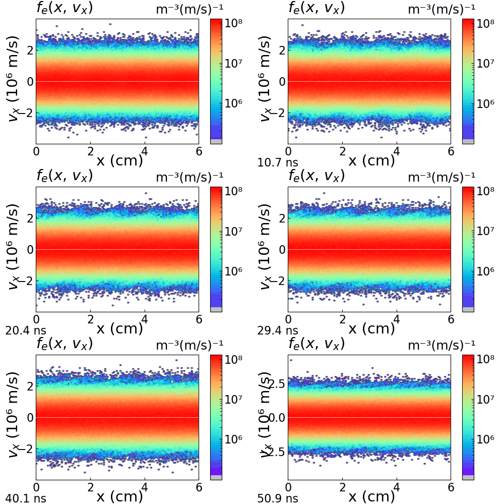
Figure 40 (animation): Electron phase space over the full run. A small coherent ripple decreases without ever trapping electrons. This is the kinetic signature of linear Landau damping.

Summary

A 2 % single-mode seed produces a textbook linear Langmuir wave. It shows a standing-wave oscillation at the exact kinetic frequency $\omega_r = 1.26\,\omega_{pe}$ (5 % above Bohm-Gross). It shows an exponential collisionless decay at the exact kinetic rate $\gamma_L = 0.053\,\omega_{pe}$ (40 % below the textbook asymptotic formula; the simulation is accurate enough to distinguish them). There are no harmonics, no trapping, and the phase space has no structure. If the seed is multiplied by fifteen, every one of these statements becomes false. That is the Large-Amplitude case.

II.D. Case 2 Large-Amplitude Langmuir Wave (Electron Trapping)

In the Bohm-Gross case a small ($2\%$) perturbation produced a clean linear oscillation that was damped smoothly by Landau damping. Here the plasma is driven strongly. A $30\%$ density perturbation creates potential wells deeper than the electron thermal energy. These wells physically trap the resonant electrons and form “cat’s-eye” vortices in phase space. These are the trapped-particle structures of the Bernstein-Greene-Kruskal (BGK) modes [27]. Landau damping is then suppressed, because the trapped electrons return energy to the wave instead of taking it away, as analysed by O’Neil [26]. The wave survives, as a slowly evolving nonlinear structure, far beyond its linear damping time.

Physics

The relevant numbers are all fixed by the conditions below. The plasma ($n_0 = 2\times 10^{14}$ m⁻³, $T_e = 3$ eV) has $f_{pe} = 127$ MHz (period $2\pi/\omega_{pe} = 7.9$ ns), $v_{th} = 7.3\times 10^{5}$ m/s and $\lambda_{De} = 0.91$ mm. Seeding mode $m = 4$ in the $L = 6$ cm periodic box gives $k = 2\pi m/L = 419$ m⁻¹, i.e. $k\lambda_{De} = 0.38$. The Bohm-Gross frequency is $\omega = 1.20\,\omega_{pe}$ (period 6.6 ns) and the phase velocity is $v_\phi = \omega/k = 2.3\times 10^{6}$ m/s $= 3.2\,v_{th}$. This velocity is in the tail of the Maxwellian, but the tail is populated. The linear Landau rate at this $k\lambda_{De}$ would be $\gamma_L \simeq 0.053\,\omega_{pe}$ (e-folding in 24 ns, the exact kinetic value established in the Bohm-Gross case).

The seed amplitude changes everything. With $\delta n/n = 0.3$, Poisson’s equation gives a wave potential $\phi_1 = (\delta n/n)\,T_e/(k\lambda_{De})^2 \simeq 6.2$ V, i.e. potential wells of depth $e\phi_1 \simeq 2.1\,T_e$. Electrons within the trapping separatrix, a band of half-width $2\sqrt{e\phi_1/m} \simeq 2.9\,v_{th}$ around $v_\phi$, cannot stream through the wave. They bounce inside the wells at the frequency

i.e. a bounce period $\tau_B \simeq 14$ ns. Since $\omega_B/\gamma_L \simeq 10$, trapping is much faster than Landau damping. After about one bounce period the resonant electrons are phase-mixed inside the wells. The net energy exchange between wave and particles stops, and the wave reaches a long-lived BGK state [27], [26]. Finally, the initial perturbation is a pure density modulation that carries no net current. It therefore splits into two counter-propagating waves of equal amplitude, that is a standing wave. The trapping structures therefore appear at both $+v_\phi$ and $-v_\phi$, and the field energy of the standing wave oscillates at $2\omega$ (period 3.3 ns).

Simulation conditions

• Plasma: uniform $n_0 = 2\times 10^{14}$ m⁻³, electrons Maxwellian at $T_e = 3$ eV; immobile ions (mass ratio overridden to $10^{6}$). This is a pure electron-wave problem on a fixed neutralizing background.
• Domain: $L = 6$ cm, strictly periodic, no collisions (zero gas pressure).
• Perturbation (Langmuir seed): at $t = 0$ each electron is displaced by $\delta x = (a/k)\sin(kx)$ with $a = 0.3$ and $k = 2\pi m/L$, $m = 4$. This is a charge-conserving density wave $\delta n/n = 0.3$ (no particle added, ions untouched). Fresh Start required.
• Numerics: 256 cells ($\Delta x = 0.23$ mm $= 0.26\,\lambda_{De}$, 64 cells per wavelength), 4000 macroparticles per cell ($\simeq 10^{6}$ total), time step $10$ ps ($\omega_{pe}\Delta t = 0.008$), run to 100 ns. History sampling every 20 steps (0.2 ns) to resolve the $2\omega$ oscillation of the field energy.

Results

Figure 41: Initial condition ($t = 0$): electron density (cyan), uniform frozen ion background (blue) and self-consistent potential (red).

The Langmuir seed produces the expected large-amplitude structure: four wavelengths of a $30\%$ density modulation. The shape is nonlinear, with sharp crests at $1.4\,n_0$ and flat troughs at $0.77\,n_0$, which is characteristic of a displacement-generated wave at large amplitude. The corresponding potential wells have a depth of $2\phi_1 \simeq 12$ V, i.e. $e\phi_1 \simeq 2\,T_e$ per well. This is deep enough to trap a substantial fraction of the electron distribution.

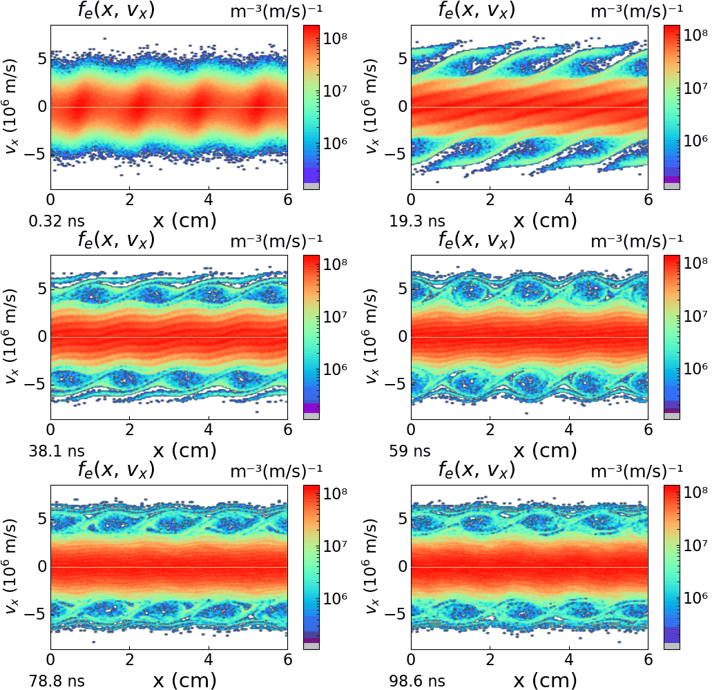
Figure 42 (animation): Electron phase space $f_e(x, v_x)$ over the full run (log color scale).

This movie shows the whole case. Within about one bounce period the resonant electrons roll up into four “cat’s-eye” vortices per side, centred at $v_x \simeq \pm v_\phi = \pm 2.3\times 10^{6}$ m/s. There is one vortex per seeded wavelength, for both signs of $v_x$, because the standing wave contains the two counter-propagating waves. The vortices are the trapped-electron orbits of the BGK mode: the electrons visibly circulate around the wave frame instead of streaming through it. At late times the vortices slowly become blurred. Electrons deep in a well bounce faster than electrons near the separatrix, so the trapped population winds into filaments (phase mixing). However, the structures are still clearly present at 100 ns, four linear damping times after the start.

Figure 43: Snapshots of the electron phase space during vortex formation ($\simeq 7$ ns $\simeq \tau_B/2$), in the mature BGK regime ($\simeq 30$ ns) and at the end of the run ($\simeq 100$ ns).

The three stages of the trapping dynamics are the following. At $\tau_B/2$ the resonant band is being folded around the wave crests (the vortices are forming). At $30$ ns the eight cat’s eyes are fully developed, and the empty separatrix clearly separates trapped electrons from passing electrons. At $100$ ns the vortices persist, but their interiors are phase-mixed into spiral filaments and the separatrix region has been filled. This is the kinetic path from a coherent wave to a quasi-stationary BGK equilibrium.

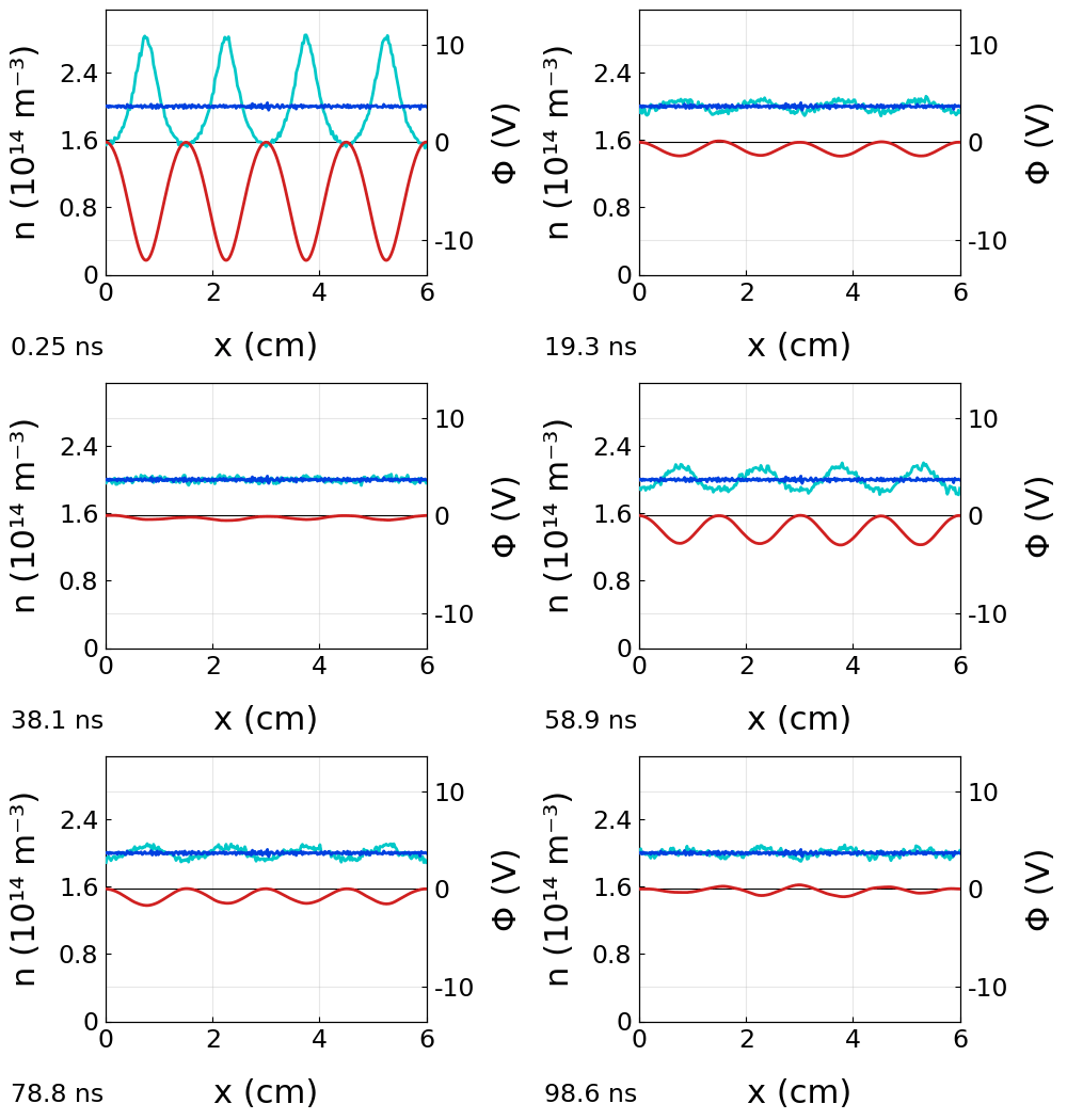
Figure 44 (animation): Charged-particle densities and potential over the run.

This is the macroscopic counterpart of Figure 42. The four-wavelength pattern oscillates in place as a standing wave: crests and troughs exchange places every half wave period, 3.3 ns. Its amplitude decreases strongly during the first bounce periods, as the wave energy is transferred to the trapped electrons. A small residual standing modulation ($\delta n/n \simeq 10\%$, $\Phi \simeq \pm 2.5$ V at 65 ns) survives. This is the field of the BGK state.

Figure 45: Electron mean energy (cyan, left axis), total kinetic energy (blue) and electrostatic field energy $U_{field}$ (purple, right axis, log scale) versus time.

The field energy is the quantitative record of the trapping dynamics. It oscillates at $2\omega$ (period 3.3 ns; a standing wave exchanges its energy with the coherent electron motion twice per wave period). Its envelope decreases by two orders of magnitude in $\simeq 20$ ns, roughly $1.5\,\tau_B$. This is not Landau damping, which would be a clean exponential decay over 24 ns. It is the violent initial transfer of energy to the trapped electrons. The envelope then increases again around 50-60 ns before it decreases again. This is the O’Neil amplitude oscillation [26], the coherent exchange of energy between the wave and the trapped population. Its period ($\simeq 40$ ns) is much longer than the initial $\tau_B$, because the bounce frequency scales as $\sqrt{\phi_1}$. With the field energy reduced by two decades, the bounce period is correspondingly longer. Meanwhile the electron mean energy (cyan) decreases from 4.8 to 4.55 eV. The coherent oscillation energy has become disordered kinetic energy, at constant total energy (blue).

Figure 46: Space-time map of the electron density over the full run.

The checkerboard pattern is the standing wave: density crests and troughs alternate in place with the half-period $T/2 = 3.3$ ns, in the four fixed cells of the $m = 4$ pattern. The amplitude decreases sharply after the first few bounce periods (the color scale saturates at early times). However, the pattern itself, that is the positions of the nodes and antinodes, remains coherent over the entire 100 ns, with only a slow drift at late times. The residual wave is not noise. It is the ordered field of the BGK state, exactly as the phase-space movie shows.

Figure 47: 2D Fourier transform $(k, \omega)$ of the density map, with the Bohm-Gross dispersion relation (dashed).

All the spectral energy is concentrated in two sharp peaks at $k\lambda_{De} = \pm 0.38$, which correspond to the seeded mode in both propagation directions. The peaks are on the Bohm-Gross parabola at $\omega \simeq 1.2\,\omega_{pe}$. Even in this strongly nonlinear regime the carrier wave still obeys the linear dispersion relation. The moderate frequency spread of the peaks reflects the amplitude decay during the measurement window and the nonlinear frequency shift of the trapped-particle wave.

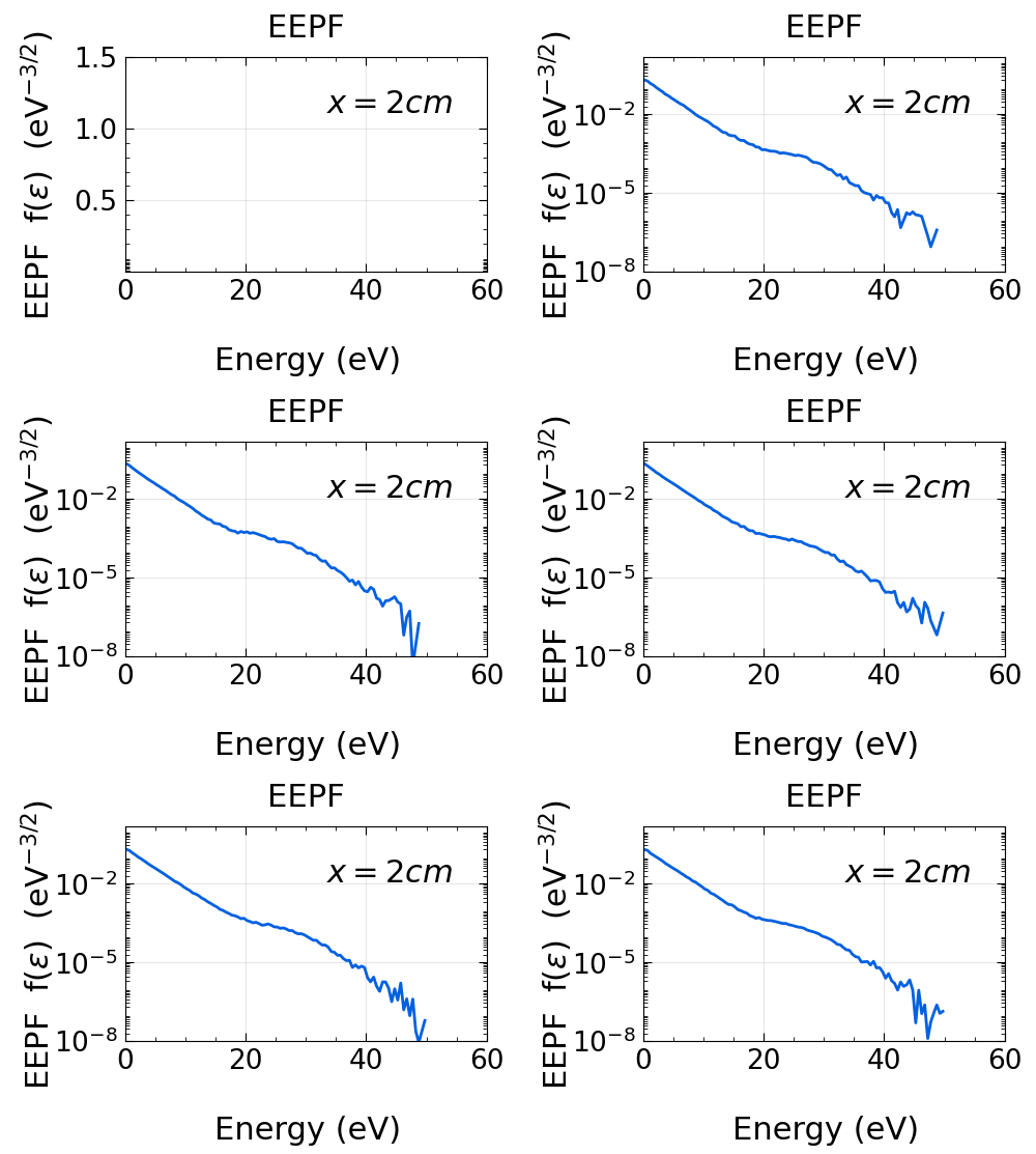
Figure 48 (animation): Evolution of the electron energy probability function.

This is the signature of trapping in energy space. The initial straight line (Maxwellian at 3 eV) develops a plateau between $\simeq 15$ and $\simeq 45$ eV, then a sharp cutoff near 50 eV. These numbers are exactly the trapping structure of the Physics section. The resonance is at $\varepsilon_\phi = \frac{1}{2}mv_\phi^2 \simeq 15$ eV. The plateau is the phase-mixed trapped population spread along the separatrix. The cutoff corresponds to the top of the separatrix, $\frac{1}{2}m(v_\phi + 2\sqrt{e\phi_1/m})^2 \simeq 55$ eV; no electron can be accelerated beyond it. The wave has irreversibly heated a small fraction of the electrons into a supra-thermal tail. This is a kinetic result that no fluid model can reproduce.

Summary

Every measured feature agrees quantitatively with the trapping theory. The vortices are centred at $\pm v_\phi = \pm 2.3\times 10^{6}$ m/s. The field energy first decreases in $\simeq 1.5\,\tau_B$. The standing wave oscillates at $T/2 = 3.3$ ns. The O’Neil envelope increases again once the bounce becomes slower because of the reduced amplitude. The EEPF plateau is bounded by the separatrix (15-55 eV). The carrier wave remains on the Bohm-Gross parabola throughout. Compared with the linear Bohm-Gross case, a single parameter was changed: the seed amplitude, from $2\%$ to $30\%$. The physics changed regime entirely, from exponential Landau damping to a long-lived, trapped-particle BGK wave.

II.E Ion Acoustic Waves (IAW)

In neutral gases, sound waves propagate through collisions between particles, which transmit local pressure variations. In a plasma, however, collective behavior allows “sound” to propagate even when there are no collisions at all. These waves are the Ion Acoustic Waves (IAW) [22,29]. They are longitudinal oscillations in which the restoring force is provided by the thermal pressure of the electrons, and the inertia is provided by the heavy ions.

In low-temperature plasmas (LTP), where the electrons are usually much hotter than the ions ($T_e \gg T_i$), ion acoustic waves are a fundamental mode of energy transport. They govern phenomena from ambipolar diffusion to the formation of shock waves.

The Physical Mechanism

Because the electrons are very light and mobile, their thermal pressure makes them expand rapidly down density gradients. As they leave the heavier ions behind, a small charge separation appears. This separation generates an ambipolar electric field that pulls the ions along, so that the ions follow the electrons. When this expansion is perturbed, the plasma oscillates. The electrons provide the “spring” (through the electric field generated by their pressure), and the ions act as the “mass” attached to that spring.

The Basic Fluid Equations

To derive the behavior of an IAW, the plasma can be described with a simplified 1D two-fluid model. The ions are assumed to be completely cold ($T_i = 0$) and to respond only to the macroscopic electric field $E = -\nabla \Phi$.

The ion fluid is governed by the Continuity and Momentum equations:

Because the electrons are hot and light, they react almost instantaneously to the potential $\Phi$. Their inertia is neglected, and they follow a thermodynamic equilibrium described by the Boltzmann relation:

Finally, the ion and electron densities are coupled by Poisson’s Equation, which gives the electric field created by the charge separation:

The Dispersion Relation

These equations are linearized (assuming small perturbations $\delta n$, $\delta v$, and $\delta \Phi$ around a uniform equilibrium state $n_0$), and wave solutions of the form $\exp(i(kx - \omega t))$ are searched for. This gives the fundamental dispersion relation for Ion Acoustic Waves [30]:

This equation depends on two important plasma parameters:

• The Ion Acoustic Speed ($c_s$): The characteristic velocity of the wave, defined only by the electron temperature and the ion mass: $c_s = \sqrt{\frac{e T_e}{m_i}}$.
• The Electron Debye Length ($\lambda_{De}$): The fundamental shielding distance in the plasma: $\lambda_{De} = \sqrt{\frac{\varepsilon_0 T_e}{n_0 e}}$.

Asymptotic Limits and Physical Regimes

The dispersion relation shows two distinct physical regimes, depending on the wavelength $\lambda = 2\pi/k$:

• Long Wavelength Limit ($k \lambda_{De} \ll 1$): When the wavelength is much larger than the Debye length, the plasma remains almost quasi-neutral ($n_i \approx n_e$). The denominator approaches $1$, and the relation becomes $\omega \approx k c_s$. In this regime the wave is non-dispersive. It travels exactly at the constant speed of sound $c_s$, like a sound wave in air.
• Short Wavelength Limit ($k \lambda_{De} \gg 1$): When the wavelength becomes comparable to or shorter than the Debye length, quasi-neutrality is no longer valid. The electrons can no longer shield the electric fields completely. The dispersion curve becomes flat, and the frequency approaches an asymptotic maximum: $\omega \approx \omega_{pi}$, where $\omega_{pi} = \sqrt{\frac{n_0 e^2}{\varepsilon_0 m_i}}$ is the ion plasma frequency. The wave can no longer transport energy effectively and becomes highly dispersive.

Moving Beyond Fluids: The Kinetic Perspective

The fluid derivation gives the structure of the wave, but it says nothing about the exchange of energy between the wave and individual particles.

For this reason a kinetic Particle-In-Cell (PIC) approach is essential. Fluid theory cannot predict Ion Landau Damping (the collisionless attenuation of the wave that occurs if $T_i$ approaches $T_e$). It also cannot describe large-amplitude nonlinear effects such as wave breaking [31], particle trapping, and the generation of supersonic ion beams. The two cases of this section show these kinetic effects directly.

II.E. Case 1 Generation of Ion Acoustic Waves

1D Kinetic Simulation of Ion Acoustic Waves

This case tests the dispersion relation given in the chapeau. We simulate the generation and propagation of ion acoustic waves [29-30] in a 1D collisionless plasma.

The Simulation Setup

The simulation is set up for a Helium plasma in a 20 cm gap at 0 Torr. The initial conditions are a uniform density $n_0 = 2 \times 10^{14}\text{ m}^{-3}$, an electron temperature $T_e = 3\text{ eV}$ and an ion temperature $T_i = 0.026\text{ eV}$. A periodic perturbation is created by injecting equal numbers of electrons and ions at the center of the gap ($x_0 = 10\text{ cm}$). The net injected charge is therefore zero. The injection takes place every 3 µs (the injection waveform repeats with a 3 µs period), for four pulses over the 11 µs run.

The source is a half-sine time pulse of duration $\tau = 100\text{ ns}$ with a spatially integrated equivalent current density amplitude $J_0 = 1\text{ A/m}^2$. The spatial profile of this injection is spread over a 4 mm width (from 49% to 51% of the gap) with a raised cosine shape: $0.5[1 + \cos(2\pi(x - x_0)/(x_2 - x_1))]$.

Since $J_0$ is the spatially integrated source, the total number of injected particles per unit area for each species per pulse is obtained by integrating over time only:

With the values above, this gives $N_{inj} \approx 3.98 \times 10^{11}\text{ particles/m}^2$. The raised cosine spatial distribution has an effective integrated width of 2 mm. The peak density perturbation at the exact center of the gap is therefore:

This peak added density is approximately equal to the background density ($\Delta n_{peak} \approx n_0$). This is a strong, localized perturbation. It drives the acoustic modes well above the PIC noise.

The Physical Mechanism of the Acoustic Pulse

To understand the generation of the wave, the microscopic thermodynamics immediately after the injection must be examined. At $x = 10\text{ cm}$, a localized, electrically neutral cloud of particles is injected. The electron temperature ($T_e = 3\text{ eV}$) is more than two orders of magnitude higher than the ion temperature ($T_i = 0.026\text{ eV}$). The electrons are therefore much faster.

Immediately after the injection, the hot electrons start to escape from the central region. The heavy, cold ions do not have the thermal velocity to follow them, and they remain behind. This rapid charge separation creates an intense, localized ambipolar electric field directed outwards from the injection center. This field pulls the escaping electrons back and, at the same time, pushes the ions outward. The ions are pushed outward by the electron pressure gradient. This starts the ion acoustic pulse, which propagates at the sound speed $c_s$.

Interpreting the Diagnostics

The simulation shows both the macroscopic, fluid-like propagation of these waves and the microscopic kinetic memory behind it.

Figure 49: Spatio-temporal evolution $(x, t)$ of the ion density. The periodic intense injections create primary “V” shaped wave trajectories. The free-streaming ions of earlier pulses go around the periodic domain and cross the fronts of later pulses. This produces the fainter criss-cross interference pattern.

Spatiotemporal Evolution and Ballistic Streaming (Figure 49)

Figure 49 gives a macroscopic view of the plasma density over time. Each major injection creates a distinct, bright “V” shape starting from the center. The constant slope of these fronts ($\Delta x / \Delta t$) is exactly equal to the theoretical ion sound speed ($c_s = \sqrt{e T_e / m_i}$).

Beyond the primary wave fronts, the plot shows a fainter criss-cross pattern. Its origin is purely kinetic and due to free streaming. The domain is periodic (there are no walls or sheaths in this run). The ions launched by each pulse are therefore not stopped anywhere. They stream ballistically at their individual velocities, go around the 20 cm box, and cross the fronts emitted by the following pulses. Where two counter-propagating groups overlap, their densities add and a faint transient crest appears. The crossing points form the criss-cross pattern. This is the macroscopic sign of ballistic phase mixing. The perturbation has not really disappeared after the primary front has passed. Its “memory” remains in the ion velocity distribution and appears again in the density whenever streams overlap. A single-fluid model, which averages over velocity, cannot reproduce this. (A true nonlinear plasma echo, the spontaneous re-appearance of a wave at a beat location from two drives at different frequencies, is a related but different effect. It is not claimed here.)

Figure 50: 2D Fast Fourier Transform of the ion density fluctuations in the $(k, \omega)$ space. The spectral energy follows the theoretical ion acoustic dispersion curve (dashed white line).

Spectral Analysis and Dispersion (Figure 50)

Figure 50 confirms the nature of these propagating structures. The $(x,t)$ density data are transformed into the spectral $(k, \omega)$ domain. The spectral energy density then agrees very well with the theoretical fluid dispersion relation for ion acoustic waves (dashed white line).

The distinct horizontal “striping” or banding visible in the spectrum is a direct consequence of the temporal periodicity of the source injections. The discrete frequency harmonics ($\omega$) are strictly fixed by the 0.33 MHz repetition rate of the perturbation (one pulse every 3 µs). The energy remains closely concentrated on the theoretical curve. This confirms that the main mechanism of energy transport is indeed the ion acoustic mode.

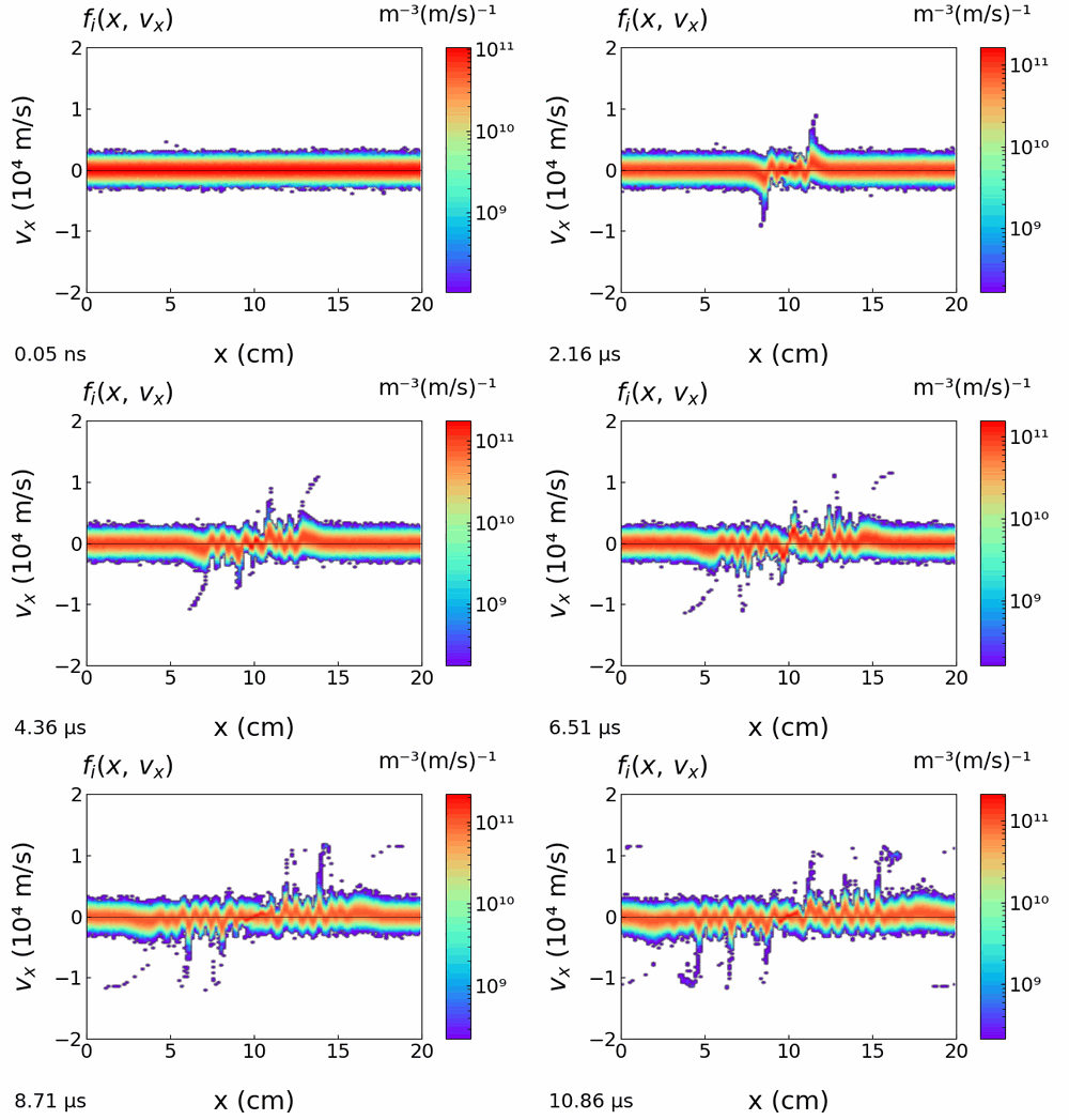
Figure 51: Time evolution of the ion phase space distribution $f_i(x, v_x)$ . It shows the acceleration of the ions and the ballistic streaming responsible for phase mixing.

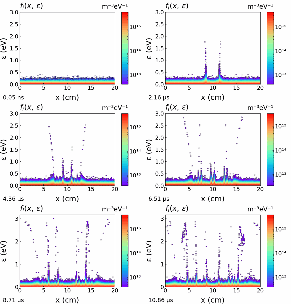
Figure 52: Time evolution of the ion phase space distribution $f_i(x, \epsilon)$.

Kinetic Dynamics in Phase Space (Figures 51 & 52)

Figures 49 and 50 show the macroscopic results. The phase-space animations for $(x, v_x)$ and $(x, \epsilon)$ show the kinetic mechanism behind them.

Initially, the plasma is at rest as a dense, flat horizontal band centered at $v_x = 0$ (and $\epsilon \approx 0.026\text{ eV}$). This band represents the cold, stationary Maxwellian background. When the pulse occurs, the ambipolar field strongly deforms this band. The animations show it locally twisted and stretched, with groups of particles sent to higher velocities and energies.

During the pulse: A fraction of the ions is accelerated to the phase velocity of the wave. This creates a strongly non-Maxwellian bump-on-tail distribution at the wave front. After the pulse: These energetic ions continue to stream ballistically across the gap. Particles with slightly different velocities travel at different speeds, so the initial narrow perturbation spreads out in space. This is the visual representation of phase mixing.

It is exactly the folding and overlapping of these ballistic ion streams in the $(x, v_x)$ phase space that produces the criss-cross density pattern of Figure 49. Single-fluid codes do not show this at all, because they average over the velocity dimension and lose the kinetic memory carried by the streams.

II.E. Case 2 Wave Breaking

Wave Breaking and Nonlinear Effects

The linear fluid regime assumes very small perturbations. However, real laboratory plasmas often involve high-power antennas, laser pulses, or intense transient localized fields. In this section, the plasma is driven into the strongly nonlinear regime [31] by increasing the amplitude of the initial electrostatic perturbation.

The linear approximation fails when the local potential well ($\Delta\Phi$) becomes so deep that the electrostatic energy transferred to the ions is larger than the electron thermal energy ($\Delta\Phi > T_e / 2$). The acoustic wave steepens into a shock, and a purely kinetic phenomenon appears: wave breaking.

The Simulation Setup

The Helium plasma configuration is the same as in the previous example ($T_e =$ 3 eV, $T_i =$ 0.026 eV). However, the amplitude of the 100 ns electrostatic pulse applied at the center ($x =$ 10 cm) is multiplied by a factor of 4. This creates a strong transient electric field that accelerates ions to supersonic speeds. In contrast with the previous example, only a single pulse is applied here.

Interpreting the Diagnostics

In this regime a single-fluid code fails or gives unphysical results. The kinetic diagnostics show what really happens.

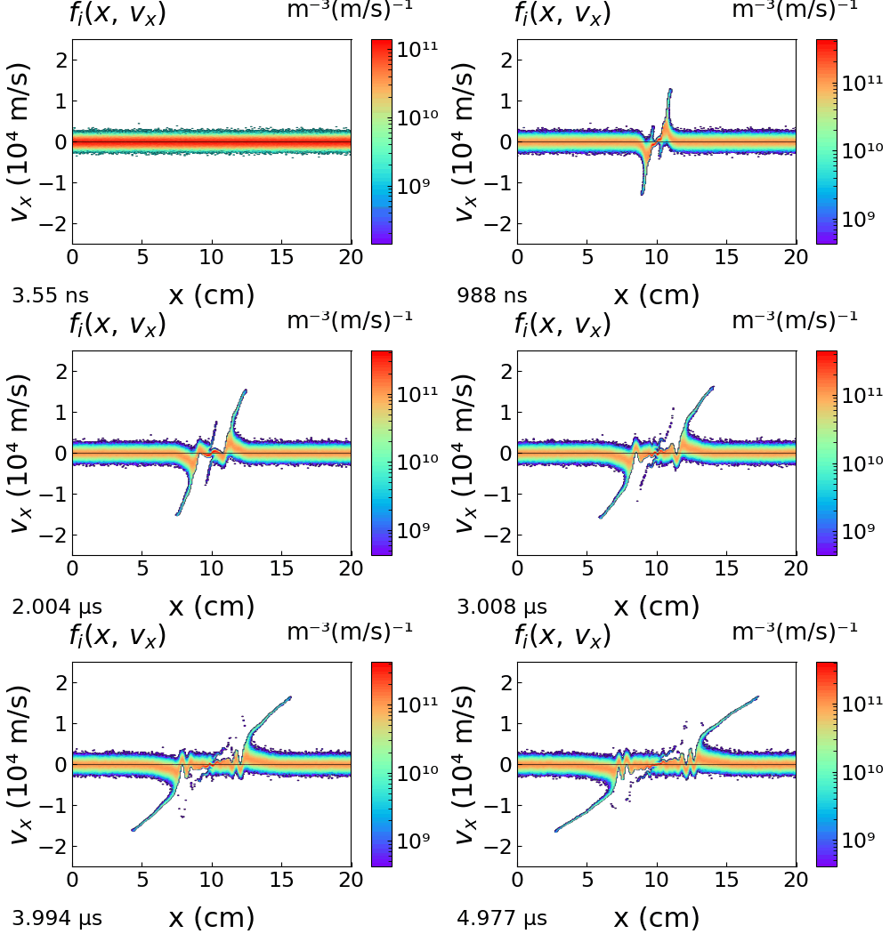
Figure 53: Ion phase space $f(x,v_x)$ during a non-linear acoustic pulse. The intense electric field accelerates a fraction of the ions to supersonic speed, so that the phase-space distribution folds over itself (multi-streaming).

Figure 54: Ion phase space $f(x,\epsilon)$ . The fast, supersonic ions reach energies larger than the electron mean energy.

1. Multi-streaming in Phase Space (Figures 53 & 54) Figure 53 shows the kinetic signature of wave breaking. In the linear regime the perturbations are small sinusoidal ripples. Here, the intense electric field accelerates part of the ions to speeds well above the local sound speed ($v \gg c_s$). This creates supersonic ion beams, or “jets”. The distribution folds. At a given position $x$ near the wave front, there are now two separate populations of ions: the stationary background ions, and the fast supersonic beam that collides with them. The presence of several velocities at the same position is called multi-streaming. This is exactly the situation in which single-fluid models fail. The evolution of the $(x,\epsilon)$ ion phase space shows that some ions in the front are accelerated to energies as large as several eV.

Figure 55: Spatio-temporal evolution $f(x,t$) of the ion density in the highly nonlinear regime. The high-amplitude perturbation creates a deep and long-lasting density rarefaction at the center, and it launches steep shock-like fronts.

2. Density Cavitation and Steepening (Figure 55) The macroscopic density evolution in Figure 55 shows clearly the effect of the strong ion expulsion. The central perturbation removes almost all the local plasma and creates a deep density “crater” (a rarefaction). This crater is refilled only slowly, as the ions drift back. The wave fronts launched outward are no longer symmetric sine waves. They steepen strongly, with sharp leading edges that are characteristic of acoustic shocks.

Figure 56: Spatial profile of the ion temperature and of its parallel and perpendicular components. There is a strong apparent parallel heating at the wave fronts and a cooling in the center.

3. Kinematic Heating vs. Adiabatic Cooling (Figure 56) The PIC code computes the temperature as the variance of the local velocity distribution ($T \propto \langle v^2 \rangle - \langle v \rangle^2$). For this reason, the nonlinear wave strongly changes the apparent thermodynamics shown in Figure 56:

Cooling at the centre: At the exact position of the pulse ($x =$ 10 cm), the parallel temperature ($T_{i\parallel}$) decreases well below the initial 0.026 eV. The electric field has expelled all the mobile ions, and only the nearly stationary ions remain. Because only the slowest ions remain in the deep density well, the local velocity variance is small. The result is a strong local cooling. Kinematic Heating at the Fronts: On the other hand, strong peaks of $T_{i\parallel}$ (here $\simeq 0.13$ eV, five times the 0.026 eV background) appear at the positions of the wave fronts. This is not true thermodynamic heating, because there are no collisions to thermalize the energy. It is kinematic heating caused by the multi-streaming seen in Figure 53. The distribution contains two widely separated velocity peaks (the cold background and the fast beam). When the PIC code computes the variance of this distribution, the variance is large, and it appears as a high local temperature. Anisotropy: The perpendicular temperature ($T_{i\perp}$) remains constant. The electrostatic wave acts only in 1D along the $x$-axis, so the transverse velocities keep their initial temperature. Without collisions, nothing changes them.

II.F Plasma Expansion: Fundamental Principles

Plasma expansion into a vacuum [32-33] appears in many contexts: astrophysics, laser-matter interaction, plasma propulsion. The expansion is not driven by ordinary mechanical pressure. It is driven by the large mass difference between electrons and ions, through the electric field that this difference creates.

The Classical Fluid Approach: The Self-Similar Solution

The electrons are extremely light ($m_e \ll m_i$), so their high thermal velocity makes them expand outward rapidly. To describe this quantitatively, the hot electrons are assumed to remain in approximate thermodynamic equilibrium, and to follow the Boltzmann relation:

This charge separation generates an ambipolar electric field $E = -\nabla \Phi$. This relation is combined with the cold ion fluid equations, and strict quasi-neutrality ($n_i = n_e$) is assumed everywhere. The result is the classical self-similar solution. For a plasma expanding into $x > 0$ for $t > 0$, the macroscopic quantities are given by:

(where $c_s = \sqrt{e T_e / m_i}$* is the ion acoustic speed).

This fluid solution contains a paradox: the density never really decreases to zero, the electric field is uniform in space, and the ion velocity increases without limit with distance.

The Kinetic Reality: Mora’s Ion Front

As shown by P. Mora [33], the fluid model fails at the low-density boundary of the plasma. In reality, quasi-neutrality cannot be maintained indefinitely. The number of electrons available to sustain the field is finite. This imposes a boundary, an ion front, beyond which there are no ions.

At this boundary, the charge separation occurs over the scale of the local Debye length ($\lambda_{De}$). This creates a sharp peak of the electric field, which accelerates the outermost ions. Mora’s kinetic model gives the analytical corrections for this front:

• Maximum Expansion Velocity: The ions do not reach infinite speeds. The driving field depends on the decreasing electron density at the boundary. For this reason the maximum velocity of the ion front increases logarithmically with time:*

(where $\text{e} \approx 2.718$* is Euler’s number and $\omega_{pi}$ is the ion plasma frequency). - The Electric Field Peak: The electric field is not uniform in space. It has a strong peak exactly at the ion front. This peak is what pulls the ions forward. Initially it scales with the Debye field $E_0 = T_e / \lambda_{De}$. As the expansion proceeds, the electron thermal energy is converted into directed ion kinetic energy, and the amplitude of this peak slowly decreases.

These effects, the front, the velocity cutoff and the multi-streaming distributions, are kinetic. A particle simulation is needed to describe them. The two cases below show them: first the free expansion into vacuum, then the same expansion in a background gas.

II.F. Case 1 Plasma Expansion in Vacuum (The Kinetic Front)

In this first example a plasma slab expands freely into vacuum, without collisions [32-33]. Everything is then driven by one mechanism: the electron pressure accelerates the ions through the ambipolar field. The kinetic effects that the fluid model does not describe can be checked directly.

The Simulation Setup

A dense “slab” of unmagnetized helium plasma is initialized in the center of an empty simulation box. The plasma has hot electrons at $T_e =$ 3 eV and cold ions at $T_i =$ 0.026 eV. The boundaries of the simulation domain absorb particles perfectly, which represents an infinite vacuum on both sides. At $t = 0$, the plasma is released and begins to expand.

Conditions of the simulation

Gas: helium, collisionless (perfect vacuum, pressure = 0) Electron temperature Tₑ = 3 eV ; ion temperature Tᵢ = 0.026 eV Simulation box: 10 cm, absorbing walls on both sides, no applied voltage Initial plasma: uniform slab, 13 mm wide, centred in the box, density n₀ = 1×10¹⁶ m⁻³ Numerical parameters: 2048 cells, ≈ 200 particles/cell, time step 2×10⁻¹¹ s, run to 0.6 µs Derived scales: Debye length λ_De ≈ 0.13 mm, ion-plasma period ω_pi⁻¹ ≈ 15 ns, ion-acoustic speed c_s ≈ 8.5 km/s (with c_s = ω_pi·λ_De)

Interpreting the Diagnostics

The diagnostics show the formation of the ambipolar field and of the supersonic ion front.

Figure 57: Spatio-temporal evolution $(x, t)$* of the ion density. The plasma slab expands outward into the vacuum. At the same time a rarefaction wave propagates inward toward the center at the ion acoustic speed.

Figure 58: Space-time map of the axial electric field. The ambipolar field is antisymmetric (it points outward on both sides). Its intense peaks (~8 kV/m) follow the two ion fronts and decrease as the expansion proceeds, according to Mora’s law E_front ∝ 1/ω_pi t.

1. Macroscopic Density and the Rarefaction Wave (Figures 57 and 58)

The density evolution in Figure 57 shows two distinct boundaries. On the outside, the plasma density extends continuously into the vacuum. On the inside, a rarefaction wave travels from the edge towards the center of the dense slab. The outer expansion is highly supersonic. The rarefaction wave, however, travels through the undisturbed quasi-neutral plasma exactly at the ion acoustic speed ($v = -c_s$). When the rarefaction waves from both sides meet at the center, the entire plasma slab enters the expansion phase, and the central density begins to decrease.

Figure 59: Ion phase space $f_i(x, v_x)$* during the expansion. The ambipolar electric field accelerates the outermost ions to highly supersonic velocities. This creates a distinct, non-Maxwellian ballistic front with a strict maximum velocity cutoff.

Figure 60: *Mean ion velocity ⟨v_x⟩_i normalised to the ion-acoustic speed c_s (here at 598 ns). The profile is linear in x (the self-similar law) and symmetric. The sharp decrease to zero at ≈ ±5.7 c_s is the finite maximum velocity, the quantity that the fluid model wrongly predicts to be infinite.*

2. The Supersonic Ion Front and Velocity Cutoff (Figures 59 and 60)

The phase space of Figure 59 is where the kinetic simulation goes beyond the fluid theory. In a fluid model, the ion velocity would simply form a straight line extending to infinity. In the PIC diagnostic, distinct “beaks” appear at the expanding edges. The ions at the very front are accelerated to velocities well above $c_s$. However, this acceleration stops abruptly and forms a clean maximum velocity cutoff. This cutoff is purely kinetic. It is determined by the finite number of electrons in the high-energy tail of the Maxwellian distribution that can maintain the charge separation at the expanding edge. As predicted by Mora’s kinetic theory, this maximum velocity does not diverge immediately but increases logarithmically with time.

Figure 61: Spatial profile of the macroscopic electric field $E(x)$*. A sharp, intense peak forms exactly at the location of the ion front. Its width scales with the local Debye length.

3. The Ambipolar Electric Field Peak (Figure 61)

The mechanism that drives the expansion is visible in Figure 61. According to the classical self-similar fluid solution, the electric field should be uniform across the expanding region. The simulation shows something different: the electric field has a strong, localized peak exactly at the ion front. This peak represents the breakdown of quasi-neutrality. The highly mobile electrons extend about one Debye length ($\lambda_{De}$) beyond the outermost ions. This thin layer of positive space charge pulls the ions forward and converts electron thermal energy into directed ion motion.

Quantitative comparison with Mora’s kinetic model

The three signatures predicted by Mora’s kinetic treatment [33] are reproduced: - Self-similar velocity. The ion velocity is linear in x, v_i = c_s(1 + x/c_s t), and symmetric about the centre (Figure 60). - Finite maximum velocity. Instead of the unbounded velocity of the fluid model, a sharp cutoff appears at the ion front. Here ⟨v_x⟩_i reaches ≈ 5.7 c_s (the true maximum, at the tip of the phase space, is slightly higher). This is consistent with Mora’s front-velocity law v_front ≈ 2 c_s ln(ω_pi t/√(2e)). - Field peak at the front. The electric field is not uniform. It has a sharp peak at the ion front (Figures 58 and 61), where quasi-neutrality breaks down over about one Debye length.

Because the slab is finite, its reservoir of electrons is slowly depleted (rarefaction time ≈ R₀/c_s ≈ 0.8 µs). The electrons cool, and the maximum ion velocity is expected to saturate at late times instead of increasing logarithmically without limit. This is the link between the semi-infinite isothermal model [33] and the finite-plasma adiabatic model [34].

Figure 62 (electron dynamics): Electron phase space f_e(x, v_x). The electrons form a hot, fast lens (velocities ~40× the ion velocities) at the same location as the ions. They are the “engine” that builds the ambipolar field. With absorbing walls the escaping high-energy tail is cleanly removed (no spurious recirculation). The plasma becomes slightly positive (plasma potential ≈ +13 V ≈ 4 Tₑ), and this sets the barrier that limits the ion energy.

II.F. Case 2 Plasma Expansion with Collisions

This case is the collisional counterpart of the previous one. The same dense helium plasma slab is left to expand between two grounded, absorbing electrodes. However, the surrounding vacuum is now replaced by a background of neutral helium at $p = 0.5$ Torr. Everything else is unchanged, so the two cases can be compared directly. The Monte-Carlo collision (MCC) module of JC-PIC now scatters both species on the neutral gas. For the ions, the main processes are $\mathrm{He^+}$–$\mathrm{He}$ charge exchange and elastic scattering; for the electrons, $e$–$\mathrm{He}$ elastic scattering. As a result, the smooth, freely accelerating self-similar rarefaction of the vacuum case is strongly modified. The neutral density ($n_g \simeq 1.6\times10^{22}$ m⁻³, about $10^{6}$ times the plasma density) is essentially unperturbed and acts as a fixed collisional background. The ionization fraction is $\sim 10^{-6}$, and no significant ionization occurs at $T_e = 3$ eV.

Simulation conditions

The conditions are identical to those of the vacuum-expansion case, with the neutral background added:

• Gas: Helium at $p = 0.5$ Torr, 300 K ($n_g \simeq 1.6\times10^{22}$ m⁻³). MCC collisions on (elastic, excitation and ionization for electrons; elastic + charge exchange for ions).
• Domain: 10 cm gap between two grounded, absorbing electrodes.
• Initial plasma: a 13 mm slab centred at mid-gap ($x/L \in [0.435, 0.565]$), density $10^{16}$ m⁻³, $T_e = 3$ eV, $T_i = 0.026$ eV.
• No source, no heating, no applied voltage: the slab is simply released and left to expand.
• Numerics: 2000 grid cells, time step down to $2\times10^{-12}$ s, run to $1.2$ µs.

Collisional regime

The mean free paths decide whether collisions are important. The helium cross sections at these energies are $\sigma_i \sim 3\text{–}4\times10^{-19}$ m² for $\mathrm{He^+}$–$\mathrm{He}$ charge exchange and $\sigma_e \sim 5\times10^{-20}$ m² for $e$–$\mathrm{He}$ elastic scattering at $T_e = 3$ eV. With these values, the mean free paths $\lambda = 1/(n_g\sigma)$ at $0.5$ Torr are about 0.2 mm for the ions and 1.2 mm for the electrons.

The ion mean free path is two orders of magnitude smaller than the initial slab (13 mm) and than the expansion length scale. The ions are therefore strongly collisional. Each ion undergoes of the order of $\nu\,t \sim (c_s/\lambda)\,t \approx 40$ charge-exchange collisions during the microsecond of the run (the sound speed is $c_s = \sqrt{eT_e/M} \simeq 8.5$ km/s for helium at $T_e = 3$ eV). The electrons are only moderately collisional ($\lambda \sim 1$ mm). This asymmetry, strongly collisional ions and weakly collisional electrons, determines all the results below. The relevant transport coefficient is now the ambipolar diffusion coefficient $D_a \simeq D_i(1 + T_e/T_i) \approx 5$ m²/s. It gives a diffusion length $\sqrt{2 D_a t} \approx 3$ mm per microsecond, which is comparable to the small edge displacement observed in the simulation.

Results

Movie 1: Charged-particle densities ($n_e$, $n_i$) and electric field $E$. At $t = 11$ ns the configuration is still the sharp initial slab, with a strong ambipolar field ($\simeq 15$ kV/m) at each edge. At this time it cannot be distinguished from the beginning of the vacuum expansion. The edges then move outward and decelerate. The front speed decreases from $\sim 9$ km/s in the first hundred nanoseconds to only $\sim 2\text{–}3$ km/s at the end. The edge field decreases ($15 \to 5 \to 3 \to 1.9$ kV/m) as the density gradient relaxes. An important point is that the field does not spread out. It remains sharply localised at the two plasma edges during the whole run and forms a quasi-stationary ambipolar double layer. By $1.2$ µs the slab has spread only from 13 mm to $\simeq 24$ mm and is almost frozen. The peak density is still near $10^{16}$ m⁻³ (in vacuum the plasma would already have expanded across the whole gap).

Figure 63: Spatio-temporal map $(x,t)$ of the ion density (last $0.6$ µs). The ion cloud is almost stationary, with two nearly vertical edges near 3.8 and 6.2 cm. This is the direct image of an expansion stopped by collisions. Charge exchange destroys the directed ion momentum almost as fast as the ambipolar field creates it, so the ion front advances very little.

Figure 64: Spatio-temporal map of the electric field. The field forms two stationary stripes, negative (pointing inward for the electrons) at the left edge and positive at the right edge, which keep their position over the whole window. This is the signature of a quasi-steady ambipolar double layer at the plasma–gas boundary. The field pushes the ions slowly outward and confines the electrons electrostatically. The two effects nearly balance, so the boundary hardly moves.

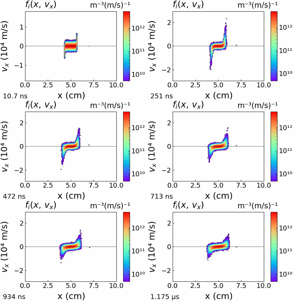
Movie 2: Ion phase space $f_i(x, v_x)$. This is the most instructive diagnostic. The self-similar rarefaction “beak” of the vacuum case is not absent: it forms and is then damped. At early times the edge ions are accelerated outward (by $\sim 400$ ns the fastest reach $\simeq 2\,c_s$), which reproduces the collisionless fan. However, charge-exchange collisions continuously convert these fast directed ions into slow ions (and fast neutrals). The tail is therefore eroded. By $1.2$ µs the fastest ions are brought back to $\simeq 1.2\,c_s$, and the whole structure is compressed near rest. The result is a strictly bounded, quasi-frozen ion distribution instead of the continuously accelerating self-similar front.

Figure 65: Mean ion velocity $\langle v_x \rangle_i$ normalised to the sound speed $c_s$, at $1.2$ µs. The main quantitative result is that the mean ion outflow never exceeds $\simeq 0.5\,c_s$: it is subsonic everywhere. In the interior, the profile is a weak antisymmetric ramp, similar to a presheath, which passes through zero at the centre. In the thin edge layers the outflow reaches a maximum of only half the sound speed, then decreases abruptly to zero outside the plasma. In the vacuum case, $\langle v_x \rangle / c_s$ became larger than unity and continued to increase towards the front. Here, the collisional drag balances the ambipolar acceleration before the ions reach the Bohm/sound speed, and this limits the expansion.

Figure 66: Ion temperatures ($T_i$, $T_{i\parallel}$, $T_{i\perp}$) at $1.2$ µs. In the quasineutral core the ions remain near their initial 0.026 eV. At the edges the parallel ion temperature increases to $\simeq 0.19$ eV (about seven times the initial value), while the perpendicular temperature remains cold. This anisotropic edge heating is produced by the mixing of ions created at different positions and times. This kinetic effect is already present in the collisionless presheath; here it is reinforced by the charge-exchange randomisation of the directed edge flow.

The electrons remain centred on the ion slab and close to Maxwellian at $T_e \simeq 3$ eV (a compact, isotropic region in phase space). Only a very small fast halo escapes towards the walls. In the vacuum case the electrons moved far ahead of the ions. Here, the $e$–$\mathrm{He}$ collisions and the confining ambipolar field keep the electron cloud essentially at the same position as the ions. This is exactly the reason why the plasma stays together and the expansion is stopped.

Discussion

Together, the diagnostics show a clear transition from the ballistic, self-similar expansion of the vacuum case to a collisional, ambipolar-confined regime. The two limits have the same beginning: the initial slab, the strong edge field, and the start of the rarefaction fan. They separate within a hundred nanoseconds. In vacuum the ion front escapes and accelerates logarithmically in time (Mora [33]). At $0.5$ Torr the ion mean free path is so short that charge exchange stops the directed motion almost immediately. The mean outflow saturates below the sound speed, and the plasma relaxes into a slowly diffusing dome bounded by a stationary ambipolar double layer. This is the collisional regime analysed by Thaury, Mora and co-workers [35]. In this regime the expansion velocity is not set by the electron temperature alone, but by the competition between the ambipolar field and the ion–neutral friction. The pressure $p = 0.5$ Torr is well inside this regime. Increasing or decreasing the pressure would move the plasma continuously between the frozen-slab limit shown here and the free vacuum expansion of the previous case.

II.G PIC-MCC and Global Model

Global models (also called volume-averaged models) are the simplest and the most widely used tools for estimating the parameters of low-temperature discharges. They reduce the plasma to a 0D description: a single density and a single electron temperature. These two quantities are obtained from a particle balance and an energy balance over the whole volume [5], [10]. Such models are the basis of the scaling laws used for reactors in plasma processing [12]. Their validity depends on strong assumptions: a quasineutral plasma with thin sheaths, a Maxwellian electron energy distribution with a temperature that is uniform in space, and simple, clearly identified channels of particle loss. A kinetic simulation is the ideal tool to test these assumptions. JC-PIC solves the same discharge with no assumption on the distribution function and no assumption on the profiles.

In this section the global model is first derived analytically for the plane-parallel (1D) geometry of JC-PIC. The derivation follows the classical treatment of Lieberman and Lichtenberg [5], [10]. The test case below then compares the predictions of the model (electron temperature, plasma density, plasma potential) with a PIC-MCC simulation in argon (4 cm gap, 50 mTorr). In this simulation a fixed power is deposited in the electrons by Maxwellian heating over the whole gap. These conditions are chosen so that the assumptions of the global model are well satisfied. The agreement is very good, and it is instructive. It shows exactly which physics the 0D model describes, and which assumptions must be accepted for that.

Principle

The model considers a plasma slab of width $l$ between two grounded (or floating) walls. The plasma is sustained in a gas of density $n_g$ by a power $P_{abs}$ absorbed by the electrons per unit electrode area. The plasma is described by only two unknowns: the central density $n_0$ and the electron temperature $T_e$ (given in eV everywhere). All the spatial structure is reduced to a single number, the edge-to-center density ratio $h_l$. Two balances close the system. The particle balance (ionization compensates the wall losses) fixes $T_e$ alone. The energy balance (the absorbed power compensates the energy carried to the walls) then fixes $n_0$.

Ion loss to the walls: Bohm flux and edge-to-center ratio As shown in the Plasma Sheath section, the ions enter the sheaths at the Bohm velocity. Each wall therefore collects the ion flux

where $n_s$ is the density at the plasma-sheath edge. The ratio $h_l$ depends on the ion transport across the gap. At high pressure the plasma is diffusive (Schottky regime): the density profile is a cosine and $h_l \simeq (\pi/l)(u_B/\nu_i)$, where $\nu_i$ is the ion-neutral collision frequency. At low pressure the profile is flat in the center and decreases near the sheath edges. A heuristic formula that connects the two regimes [5], [11] is widely used:

where $\lambda_i = 1/(n_g \sigma_i)$ is the ion-neutral mean free path ($\sigma_i \simeq 10^{-18}$ m² for Ar⁺ in argon, mainly due to charge exchange).

Particle balance: the electron temperature In steady state the ionization in the volume must compensate exactly the loss of electron-ion pairs to the two walls:

where $K_{iz}(T_e)$ is the ionization rate coefficient averaged over the Maxwellian distribution. The density $n_0$ cancels. This is the main property of the particle balance, and it leaves an equation for $T_e$ only:

The electron temperature is therefore fixed by the product $n_g d_{eff}$ (gas, pressure and size). It is independent of the absorbed power and of the plasma density. For a Maxwellian distribution in argon a convenient fit is $K_{iz} \simeq 2.34\times 10^{-14} T_e^{0.59} \exp(-17.44/T_e)$ m³/s [5]. $K_{iz}$ increases exponentially with $T_e$, while $u_B$ varies slowly. For this reason $T_e$ depends only logarithmically on $n_g d_{eff}$ and remains in the narrow range 2-5 eV for all practical conditions.

Energy cost of an electron-ion pair Each electron-ion pair lost to a wall has cost a well-defined amount of energy. This energy is usually separated into three contributions (all in eV):

The collisional cost $\varepsilon_c$ is the energy spent in the gas per ionization event. It includes the ionization energy itself, the excitation collisions that lose energy without ionizing, and the small elastic energy transfer to the atoms:

For argon ($\varepsilon_{iz} = 15.76$ eV, $\varepsilon_{ex} \simeq 12.1$ eV) $\varepsilon_c$ decreases quickly when $T_e$ increases. At low temperature there are very many excitation events per ionization and $\varepsilon_c$ reaches several hundred eV. At $T_e \simeq 2$-$4$ eV it is a few tens of eV [5], [10]. The electron kinetic cost $2T_e$ is the mean kinetic energy carried through the sheath by each electron that escapes (the flux-averaged energy of a Maxwellian). The ion cost is the energy gained by an ion that falls from the plasma to the wall: $T_e/2$ in the presheath, plus the sheath drop $V_s = (T_e/2)\ln(M/2\pi m)$ derived in the Plasma Sheath section. For argon this gives

Power balance: the plasma density In steady state the absorbed power per unit area must be equal to the energy flux to the two walls, which is $\varepsilon_T$ eV per pair lost:

This gives the central density:

The structure of the model is therefore very simple: the particle balance gives $T_e$ (independent of the power), then the power balance gives $n_0$, which is proportional to the absorbed power. All the scaling laws of low-pressure discharges follow from this. $T_e$ decreases slowly when the pressure or the gap increases. At fixed power the density increases when $\varepsilon_T$ decreases (higher $T_e$, fewer excitation events per ionization), and it also increases when the losses are more confined (smaller $h_l u_B$).

Assumptions, and what the test case checks

The derivation above uses: (i) a Maxwellian EEPF with uniform $T_e$ (used in $K_{iz}$, in the $2T_e$ electron loss and in the sheath drop $V_s$); (ii) quasineutrality with thin collisionless sheaths and the Bohm criterion; (iii) a single positive ion species, no stepwise ionization through metastables, no volume recombination; (iv) an edge-to-center ratio $h_l$ given by the heuristic formula. None of these assumptions is exact in a real discharge. In particular the EEPF of low-pressure discharges is usually NOT Maxwellian (see the other sections of this library), and stepwise ionization can be dominant at high density.

The test case of this section is built so that these assumptions are satisfied as well as possible. The conditions are argon, a 4 cm gap, 50 mTorr, and a fixed absorbed power deposited by Maxwellian heating applied over the whole gap. The heating drives the EEPF towards a Maxwellian at a prescribed rate. It represents an idealized heating mechanism and it ensures assumption (i). The comparison then concerns the quantities predicted by the global model. These are the electron temperature, the central density, the plasma potential ($\simeq V_s + T_e/2$ above the walls), the ion flux and the mean ion impact energy at the electrodes, and the terms of the power balance. All these quantities are measured self-consistently by JC-PIC.

II.G. Case 1 Global Model

In this test case a JC-PIC simulation is compared, quantity by quantity, with the analytical global model [5] derived in the section text above. The conditions are chosen so that the assumptions of the 0D model are satisfied as well as possible. The gas is argon at 50 mTorr in a 4 cm gap (diffusive ion transport, thin sheaths). A fixed power is deposited in the electrons by Maxwellian power deposition over the whole gap. This heating continuously drives the electron distribution towards a Maxwellian, which is the central assumption of the model. The comparison shows that the two balances of the global model (particle balance → $T_e$, power balance → $n_0$) reproduce the kinetic results within 5-20 %. It also identifies precisely the origin of the remaining differences (slight depletion of the EEPF tail, collisional sheaths).

Physics

Only the two results of the global model established in the section text are recalled here (plane-parallel geometry, gap $l$, gas density $n_g$). The particle balance (volume ionization = Bohm flux to the two walls) fixes the electron temperature, independently of the density and of the power:

and the power balance then fixes the density, which is proportional to the absorbed power:

Numerical application to the present conditions ($n_g = 1.61\times 10^{21}$ m⁻³ at 50 mTorr, 300 K; $l = 4$ cm; $P_{abs} = 10$ W/m²). The measured ion mean free path is $\lambda_i \simeq 0.5$ mm (Figure 73 below), so $h_l \simeq 0.13$, $d_{eff} \simeq 15$ cm and $n_g d_{eff} \simeq 2.4\times 10^{20}$ m⁻². The particle balance, with the Maxwellian argon fit $K_{iz} \simeq 2.34\times 10^{-14} T_e^{0.59} \exp(-17.44/T_e)$ m³/s, then predicts $T_e \simeq 2.2$ eV. The energy cost per electron-ion pair at this temperature, calculated with the argon cross sections of JC-PIC, is $\varepsilon_T \simeq 90$-$95$ eV (see the power balance below for its exact decomposition). The power balance then predicts $n_0 \simeq 1.0\times 10^{15}$ m⁻³. Finally, the plasma potential should be $\Phi_p \simeq \varepsilon_i \simeq 5.2 T_e \simeq 13$ V. These are the numbers to remember when reading the figures.

Simulation conditions

• Gas: Argon at 50 mTorr, 300 K ($n_g = 1.61\times 10^{21}$ m⁻³).
• Domain: 4 cm gap between two grounded, absorbing electrodes.
• Initial conditions: uniform plasma density 10¹⁵ m⁻³, $T_e = 2$ eV, $T_i = 0.026$ eV.
• Electron heating: Maxwellian power deposition, $P_{abs} = 10$ W/m² uniformly over the whole gap, with a Maxwellianization frequency of 20 MHz (each electron is re-drawn from a Maxwellian about every 50 ns; the temperature of that Maxwellian is not imposed, it adjusts locally so that the prescribed power is deposited).
• Collisions: JC-PIC argon cross sections (elastic, excitation, ionization; ion elastic + charge exchange); no electron-electron Coulomb collisions.
• Numerics: 200 grid cells ($\Delta x = 0.2$ mm), 250 macroparticles per cell initially (50000), time step $5\times 10^{-11}$ s, run to $\simeq 200$ µs.

Results

Figure 67: Spatial profiles of the electron mean energy and ionization frequency at steady state.

The electron mean energy is very uniform, $\varepsilon_e \simeq 3.8$ eV across the whole quasineutral plasma. The ionization frequency is also uniform, $\nu_{iz} \simeq 3\times 10^{4}$ s⁻¹ (the scale is logarithmic). The discharge therefore really behaves as a 0D system, and this is why the volume-averaged description is meaningful. The ionization frequency is exactly the value required by the particle balance. The mean confinement time of an electron-ion pair is $\tau = \langle n \rangle l / (2h_l n_0 u_B) \simeq 37$ µs. Its inverse, $2.7\times 10^{4}$ s⁻¹, is equal to the measured $\nu_{iz}$.

Figure 68: Spatial profiles of the total, parallel and perpendicular electron temperatures.

The electron temperature is uniform and isotropic, $T_e \simeq 2.55$ eV $= \frac{2}{3}\varepsilon_e$. The Maxwellian heating is an idealized heating that leaves no spatial or directional signature. The global model predicted $T_e \simeq 2.2$ eV: the PIC value is about 15 % higher. This is the level of agreement to expect, and the sign of the difference is understood. It comes from the small deviation of the EEPF from a Maxwellian (next figure). The difference is strongly reduced by the exponential sensitivity of $K_{iz}$. A 15 % error on $T_e$ corresponds to a factor ~2 on $K_{iz}$. The logarithmic dependence of the balance absorbs this factor easily.

Figure 69: Space-averaged electron energy probability function (EEPF) at steady state.

On this semi-logarithmic plot a Maxwellian is a straight line. The EEPF is indeed very close to a straight line of slope $\simeq 2.5$ eV over the thermal bulk. This validates the assumption of the model. Above the inelastic thresholds of argon ($\simeq 11.6$ eV for excitation, 15.76 eV for ionization) the tail is slightly depleted. The electrons that reach these energies lose them in inelastic collisions faster than the 20 MHz Maxwellianization can refill the tail. A depleted tail ionizes less than a true Maxwellian at the same temperature. This is precisely why the discharge reaches a $T_e$ slightly above the prediction of the model, which is based on a Maxwellian.

Figure 70: Charged particle densities and plasma potential at steady state.

This is the central quantitative test. The density profile is close to a cosine. This is the diffusive (Schottky) shape expected at 50 mTorr, in contrast with the flat-top profiles of the collisionless cases of this library. The peak density is $n_0 \simeq 0.97\times 10^{15}$ m⁻³. The power-balance prediction was $n_0 \simeq 1.0\times 10^{15}$ m⁻³: the agreement is within a few percent. The plasma potential is $\Phi_p \simeq 14.7$ V, to be compared with $5.2 T_e \simeq 13.3$ V calculated with the measured $T_e$. The small excess is the ambipolar potential drop across the collisional bulk, which the 0D model includes in the presheath. The wall flux gives a direct check of the edge-to-center ratio: $\Gamma_{wall}/(n_0 u_B) = 0.14$ per wall, compared with $h_l = 0.13$ from the heuristic formula.

Figure 71: Spatial profiles of the space charge and electric field at steady state.

The bulk is quasineutral (the space charge fluctuates around zero at the level of the PIC noise). It supports only the weak ambipolar field that drives the ion flux outward. The positive space-charge sheaths are $\simeq 2$ mm thick, a few Debye lengths ($\lambda_{De} \simeq 0.4$ mm at the center). The field reaches $6\times 10^{3}$ V/m at the electrodes. The thin-sheath assumption of the model ($2s \ll l$) is well satisfied.

Figure 72: Spatial profiles of the total, parallel and perpendicular ion temperatures.

In the bulk the ions remain at the gas temperature. The apparent parallel “temperature” increases to $\simeq 1.6$ eV close to the electrodes. In the sheaths and presheaths the ion flow is accelerated, but at 50 mTorr the sheaths are collisional ($\lambda_i \simeq 0.5$ mm, smaller than the 2 mm sheath width). Charge-exchange collisions constantly replace fast ions by slow ions created from the neutral gas. The resulting mixture of slow new ions and accelerated ions appears as a large velocity spread. This has a direct consequence on the energy balance, visible in the power balance below.

Figure 73: Measured collision frequencies and mean free paths (central 20 % of the gap).

This panel gives the microscopic inputs used in the application of the model. The total ion mean free path is $\lambda_i = 0.51$ mm (dominated by charge exchange and isotropic elastic scattering), which gives $h_l \simeq 0.13$. The electron frequencies are: elastic $1.2\times 10^{8}$ s⁻¹, excitation $1.6\times 10^{5}$ s⁻¹, ionization $3.5\times 10^{4}$ s⁻¹. The ratio $\nu_{ex}/\nu_{iz} \simeq 4.7$ means that each ionization is accompanied by about five excitation events. This is the dominant term of the collisional cost $\varepsilon_c$. Also, $\lambda_i/l \simeq 0.013$ (diffusive ion transport, as assumed) while $\lambda_e/l \simeq 0.23$.

Figure 74: Power balance at steady state (W/m², time-averaged).

The balance closes to $4\times 10^{-4}$ W/m²: the injected 9.94 W/m² ($= P_{abs}$) is fully accounted for. Each channel is divided by the pair creation rate ($6.7\times 10^{17}$ m⁻²s⁻¹, Figure 75). This converts it into eV per electron-ion pair and gives the measured decomposition of $\varepsilon_T$. The total is $\varepsilon_T = 93$ eV. It contains $\varepsilon_c = 75$ eV of collisional losses (consistent with $\varepsilon_{iz} + 4.7 \varepsilon_{ex} +$ elastic $\simeq 15.8 + 55 + 0.4$ eV). It contains 3.6 eV carried to the walls by the escaping electrons (slightly below the Maxwellian value $2T_e = 5.1$ eV, again because of the depleted tail). It contains 14.1 eV per pair given by the field to the ions ($\simeq e\Phi_p$, as required). The ion term of the model, $\varepsilon_i \simeq 5.2T_e = 13$ eV, is therefore correct as an energy cost. But the kinetic simulation shows where that energy really goes. Only 5.1 eV reach the electrodes (“Wall loss, ions”). 9.0 eV are deposited in the neutral gas by ion-neutral collisions in the collisional sheaths and presheaths (“Collision loss, ions”). The 0D model cannot make this distinction, but it gives the correct total.

Figure 75: Particle balance at steady state (time-averaged).

The particle balance window verifies the first equation of the global model directly. The volume ionization rate ($6.70\times 10^{17}$ m⁻²s⁻¹) is equal to the wall losses ($6.78\times 10^{17}$ m⁻²s⁻¹) to about 1 %, for electrons and for ions. The loss is ambipolar and there is no other channel: no volume recombination, no secondary emission in this run. The residual $dN/dt$ is the slow end of the initial relaxation.

Figure 76: Time evolution of the number of macro-electrons and macro-ions.

Starting from the initial guess ($10^{15}$ m⁻³ uniform), the discharge relaxes to its self-consistent steady state in a few tens of microseconds. The time scale is the ambipolar confinement time computed above ($\tau \simeq 20$-$40$ µs), and a diffusive system needs a few $\tau$ to converge. This is the same behaviour as in the Collisional Plasma Diffusion case. At steady state the particle count is stationary. This is when the balances of Figures 74 and 75 (and the comparison with the global model) are meaningful.

Summary

When its assumptions are satisfied (near-Maxwellian EEPF, imposed here by the heating; diffusive ion transport; thin sheaths), the global model is quantitatively excellent. $T_e$ is predicted within 15 % (2.2 eV vs 2.55 eV measured; the difference is explained by the slight tail depletion of the EEPF). The central density is predicted within 5 % ($1.0\times 10^{15}$ vs $0.97\times 10^{15}$ m⁻³), the plasma potential within 10 % (13.3 vs 14.7 V), and the edge-to-center ratio $h_l$ within 10 % (0.13 vs 0.14). The full energy balance $\varepsilon_T = \varepsilon_c + 2T_e + \varepsilon_i$ is verified term by term. The kinetic simulation adds what a 0D model cannot give: the shape of the EEPF and its depleted tail, the profiles, and the fate of the ion energy in the collisional sheaths.

III Swarm Physics

A swarm is a population of charged particles drifting through a neutral gas under a uniform electric field. The population is dilute enough that the particles never interact with one another and never perturb the gas. It is the simplest situation in which electron-molecule collisions can be studied quantitatively. It is also the situation in which almost everything known about those collisions has been measured. Because the gas is not perturbed, a swarm depends on a single parameter, the reduced electric field $E/N$: changing the gas density at fixed $E/N$ only rescales the lengths and the times.

What Characterises a Swarm

The macroscopic quantities that describe a swarm are its transport and rate coefficients. They are the input that a fluid model of a discharge needs. They are also the benchmark that a set of cross sections must reproduce before it can be trusted.

• the drift velocity $W$, with two distinct definitions. The flux drift velocity is the mean velocity of the particles; the bulk drift velocity is the velocity of the centroid of the density profile. They differ as soon as ionization or attachment is present, because those processes act more strongly on one part of the distribution than on another.
• the diffusion coefficients $D_L$ and $D_T$, longitudinal and transverse with respect to the field. In a swarm they are not equal, because the field breaks the isotropy. Their ratio is one of the most direct signatures of a non-Maxwellian distribution.
• the mobility $\mu$ and the characteristic energy $D_T/\mu$, historically the first measurable quantity related to the mean electron energy.
• the Townsend ionization coefficient $\alpha/N$ and the attachment coefficient $\eta/N$, which govern breakdown, together with the reduced field at which the two are equal, that is, the critical field of the gas.
• the rate coefficients of each individual collision process, which are what a chemistry model needs.

Behind every one of them is the electron energy distribution function, of which they are moments. That distribution is never Maxwellian in a swarm. Most of the difficulty of the subject, and also most of its interest, follows from this single fact.

Two Ways of Obtaining Them

Historically the coefficients were measured, in drift-tube experiments [36]. Electrons are released at one electrode, they cross a gap in a uniform field, and a quantity is recorded at the other end. This quantity is the arrival time of a pulse, the shape of a current transient, or the total current as a function of the gap length. The cross sections themselves were then largely obtained by inverting those measurements. For this reason swarm data and cross-section databases are two views of one body of knowledge, not two independent ones [37].

They can also be computed, by solving the Boltzmann equation for the electron distribution in a uniform field from a given set of cross sections [38]. This is the direction taken by a modeller, and it is what turns a database into the input of a discharge simulation.

What This Chapter Contains

JC-PIC does both, and the chapter is organised in the same way.

Collisions and Cross Sections This is the data that every swarm calculation starts from, and the algorithm that turns it into collisions. The section itself is in the Appendix, next to Single-Particle Motion. It appears here because nothing in this chapter can be read without it. A swarm parameter is an average over the cross sections shown there, and the null-collision method described there is what the swarm solver uses to sample them. It is entirely interactive, with no run to launch.

Calculation of Swarm Parameters The dedicated swarm mode of JC-PIC is an autonomous Monte Carlo solver of the Boltzmann equation, with no grid, no Poisson equation and no ions. It is used here for its original purpose: producing the coefficients from a set of cross sections. One case documents a complete sweep in neon and ends with the coefficient that decides whether a plasma remains uniform. The other verifies the solver against the MCIG reference code of Hagelaar [39] in five gases, and contains the detailed description of the method.

Swarm Experiments This is the opposite view. The 1D particle-in-cell mode is used to simulate the drift tubes themselves, with their electrodes, their finite length, their injected current and their space charge, and to examine what the measurement really returns. There are three cases: the pulsed and the steady-state Townsend experiments, and the Franck-Hertz experiment. Seen from gaseous electronics rather than from atomic physics, the Franck-Hertz experiment is a steady-state Townsend discharge operated below the ionization threshold.

The two parts answer different questions and are meant to be read together. The swarm mode gives the coefficients of an infinite, uniform, fully relaxed swarm, which is the idealisation that a fluid model needs. The 1D cases show that a real drift tube is never entirely in that state. Near the cathode the distribution is still relaxing, near the anode it is truncated by absorption, and the coefficient returned by a measurement is an average over those non-equilibrium regions. Quantifying that difference is one of the things a particle simulation can do that neither the experiment nor the equilibrium calculation can do alone.

III.A Collisions and Cross Sections

→ Go to Collisions and Cross Sections

III.B Calculation of Swarm Parameters

Given a set of cross sections, the task is to produce the transport and rate coefficients over a range of reduced field, with a quantified uncertainty on every number [36]. This is the whole content of this sub-section. It is the operation that turns a cross-section database into the input of a fluid model of a discharge [37].

Two Families of Solvers

This requires solving the Boltzmann equation for the electron distribution function in a spatially uniform field. Two families of methods are in use. They differ in what they assume, not in what they claim to compute.

The two-term expansion solvers, of which BOLSIG+ [38] is the standard, expand the distribution in Legendre polynomials of the velocity direction and keep only the first two terms. They are extremely fast and accurate over most of the parameter range. The cost is that they assume a nearly isotropic distribution and treat anisotropic scattering only through an effective momentum-transfer cross section. The error they make cannot be estimated from within the method itself. This is why a reference calculation from the other family is needed.

Monte Carlo simulation makes no such assumption. A large number of electron trajectories are followed through their collisions, and every coefficient is evaluated as an empirical average over the ensemble. The distribution function, including its anisotropy and the far tail that controls ionization, is a result of the calculation and not an assumption. The anisotropy is treated exactly, however strong it becomes. The cost is statistical noise. For this reason a Monte Carlo result has a meaning only when it comes with an error bar.

The Swarm Mode of JC-PIC

JC-PIC contains a dedicated swarm mode for exactly this purpose. It is not the particle-in-cell engine with the spatial grid switched off. It is an autonomous solver that branches at start-up and never enters the PIC initialisation. There is no grid, no Poisson equation, no ions, no walls and no spatial resolution at all. There is only an ensemble of electrons in a uniform imposed field, followed until its distribution has relaxed to the steady state. After that, every coefficient is measured as a moment of the ensemble. The swarm mode calls the same collision routines as the discharge simulations of the other chapters. This is the main reason why it exists: the coefficients tabulated here have to be consistent with the collisions the code actually performs elsewhere.

Three features of the implementation should be known before reading either case.

• Replicas rather than one long run. The ensemble is split into statistically independent replicas of a few thousand electrons, one per thread, each with its own random-number stream. The estimate is the mean over the replicas that have accumulated, and the error bar is their spread divided by $\sqrt{k}$. This is an entirely empirical uncertainty, with no assumption about the shape of the distribution. The number of replicas that must have contributed before a field value is declared converged is fixed by the solver and not by the machine. More cores reduce the wall-clock time; they do not change the accuracy.
• A sweep, not a series of independent runs. A list of reduced fields is followed downwards. Each point starts from the relaxed velocity distribution of the point above, so only the first point needs a full relaxation from a cold start. The direction is important: a hot swarm cools quickly when the field is lowered, whereas heating a cold swarm up to the next field is the slow direction, and the relaxation time increases as the field decreases.
• Convergence targets that are checked, not assumed. A point stops once the relative statistical error is below its target. The targets are separate for the mean energy, the drift velocity and the diffusion coefficients, because these quantities converge at very different rates and must not share a single criterion. The residue of the power balance, computed independently from the measured rate coefficients, then checks that the sampled state really is the steady state and not a slowly drifting one.

The Two Cases

The two cases are complementary: the first uses the solver on a question of physics, the second shows that its answers can be trusted.

Swarm Parameters in Neon A complete sweep of the reduced field in an atomic gas, from 40 to 400 Td. Neon is the simplest interesting choice and a deliberately extreme one. Elastic collisions with a neon atom remove almost none of the electron energy, and the first inelastic channel opens only at 16.6 eV. The swarm therefore has almost no way of cooling and becomes very hot: tens of electron-volts at fields where a molecular gas would still be below one electron-volt. The case documents the full coefficient table, the distribution function behind it and the statistical quality of both. Its second half is devoted to the Dufour coefficient $\chi_e$, the electron energy flux driven by a density gradient. The sign of this coefficient decides whether a plasma stays uniform or forms striations. Because it is the near-cancellation of two large terms, it needs about three hundred times more sampling than the coefficients it is built from. It is also where this calculation disagrees, by a factor of three and by the sign of a slope, with a multiterm Boltzmann solution recently published for the same gas at the same pressure.

Comparisons with MCIG The verification of the solver against MCIG [39], the Monte Carlo swarm code released by Hagelaar in 2025 as a companion to BOLSIG+. The swarm mode follows the method of this code. Three figures of that paper are reproduced in five gases (neon, argon, nitrogen, oxygen and carbon tetrafluoride), whose physics ranges from a Ramsauer minimum to a large number of vibrational channels, over three decades of reduced field. The figures are the mean energy, the ionization and attachment rate coefficients, and the first four Legendre components of the velocity distribution in nitrogen at 100 Td. This last case is the one in which the two-term expansion is known to fail, and the failure can be observed here directly. This case also carries the detailed description of the method: sampling at tentative collisions rather than at fixed times, the renormalization scheme that keeps the number of simulated particles constant despite ionization and attachment, diffusion obtained from displacements rather than from positions, and the amount of growth above which a diffusion coefficient can no longer be measured.

III.B. Case 1 Swarm Parameters in Neon

This case uses the swarm mode of JC-PIC for its basic purpose: from a set of electron-neon cross sections, compute the full table of transport and rate coefficients as a function of the reduced field, with a statistical error on every number. Neon is a simple but extreme gas. In an elastic collision an electron loses only a fraction $2m_e/M \simeq 5.4\times10^{-5}$ of its energy, and the first inelastic process starts at 16.6 eV. A neon swarm therefore has almost no way to lose energy at low field, and it becomes very hot: the mean energy is tens of eV at reduced fields where a molecular gas would be below 1 eV. Most of the results below follow from this fact.

The Calculation

The solver follows a group of electrons in a uniform and constant electric field until their velocity distribution is stationary, then computes each coefficient as an average over the electrons. There is no spatial grid, no Poisson equation and no ions. This is a Monte Carlo solution of the Boltzmann equation, with the method of the MCIG code [39].

• Gas: neon at 300 K. Cross sections from the SIGLO database on LXCat [40], as distributed with the code: one elastic momentum-transfer cross section, six excitation processes (thresholds 16.62, 16.67, 16.84, 18.72, 20.00 and 20.65 eV) and ionization (21.56 eV).
• Reduced field: 39 values of $E/N$ from 20 to 400 Td in steps of 10 Td, computed in one run.
• Field sweep: the 39 values are computed in descending order with the warm-start option. Each replica starts at the highest field and uses its stationary distribution as the starting point for the next, lower field. Only the first point needs a full relaxation from a cold start. The order matters because the relaxation time increases when the field decreases: the 20 Td point alone took a fifth of the whole sweep.
• Statistics: each $E/N$ is computed by 48 independent replicas of 2000 electrons, one per thread, all running at the same time; a field value is finished when all 48 replicas have reached the tolerance. The result is the mean over the replicas and the error bar is their standard deviation divided by the square root of 48. This error is empirical: no assumption on the distribution enters it. The number of replicas is a setting of the run, not of the hardware: a machine with fewer cores runs them in several waves and gives the same statistics.
• Convergence: each replica first relaxes over ten energy-relaxation times, then takes up to 5000 samples. A field value stops when the relative error is below 0.05 % on the mean energy and the drift velocity, and below 0.1 % on the two diffusion coefficients. All 39 values converged. The power balance closes to 0.56 %. The whole sweep took 570 s on 48 threads.
• Ionization treatment: the conservative mode is used: an ionizing collision takes the ionization energy from the electron but creates no new electron, so the swarm neither grows nor decays. In this mode the bulk and flux coefficients are equal, which is used below as a check. Ionization is small at low field but not at high field: its rate reaches 9 % of the momentum-transfer rate at 400 Td, and above about 200 Td the growth of a real swarm changes the bulk coefficients by several percent (Fig. 10 of Ref. [39]). The growth modes are the subject of the Pulsed Townsend and Steady-State Townsend cases of the next sub-section.
• Random numbers: the generator is set to SplitMix64, because a swarm run uses more random numbers than the $2^{32}$ period of the default generator.

Mean Energy and Temperatures

Figure 77: Mean electron energy and the temperatures obtained from the velocity moments, as functions of the reduced field. $T$ is the total temperature, $T_\parallel$ and $T_\perp$ its components along and across the field.

The swarm is hot. The mean energy is 8.4 eV at 20 Td, 9.8 eV at 40 Td and 33.4 eV at 400 Td. A molecular gas at the same reduced field would be about ten times colder, because rotational and vibrational excitation let the electrons lose energy at a few tenths of an eV. In neon there is nothing between the elastic collisions, which take almost no energy, and the excitation threshold at 16.6 eV.

The ratio $\langle\varepsilon\rangle / \frac{3}{2}T$ is exactly 1 for a Maxwellian distribution. Here it is 1.002 at 20 Td and 1.033 at 400 Td. This does not mean that the distribution is Maxwellian (Figure 79 shows that it is not); it means that its second and third moments keep the Maxwellian relation. The anisotropy $T_\parallel/T_\perp$ increases steadily, from 1.003 at 20 Td to 1.081 at 400 Td: the field gives energy to the parallel direction faster than the collisions redistribute it.

The Transport and Rate Coefficients

The solver produces twenty-one coefficients for each field value. The main ones are:

Table 1: the main transport and rate coefficients, in the layout of the Tables window of the code. Bulk values; the drift velocity is given as a magnitude.

Three points need a comment. The reduced mobility decreases with the field, from 3.40 to 1.52 × 10²⁴, because the momentum-transfer cross section of neon increases with energy in this range [36]. The drift velocity therefore increases more slowly than the field. The diffusion is anisotropic: $D_L/D_T$ stays between 0.64 and 0.77 over the whole range. This is a kinetic result, which a two-term expansion gives only approximately, and it is the reason why a swarm cannot be described by a single diffusion coefficient. The characteristic energy $D_T/\mu$, the quantity measured by the early drift-tube experiments, increases from 6.8 to 22.5 eV. It is close to, but not equal to, $\frac{2}{3}\langle\varepsilon\rangle$.

The relative errors over the 39 field values are 0.017 to 0.028 % on the mean energy, 0.016 to 0.034 % on the bulk drift velocity and mobility, and 0.04 to 0.12 % on the two diffusion coefficients. The flux drift velocity is noisier, 0.07 to 0.56 %, because it is an instantaneous average, while the bulk velocity comes from the displacement of the centre of the swarm over a long time.

Figure 78: Reduced rate coefficients as functions of the reduced field. Open circles: momentum transfer; filled squares: ionization; thin lines: the six excitation processes.

The momentum-transfer rate depends little on the field, from 3.9 to 8.0 × 10⁻¹⁴ m³s⁻¹, because the elastic cross section of neon varies slowly with energy. This is why the mobility varies so little. The ionization rate increases from 3.4 × 10⁻¹⁸ to 7.4 × 10⁻¹⁵ m³s⁻¹, a factor of more than two thousand, while the mean energy increases only by a factor of 4. The ionization rate is set by the electrons above 21.6 eV, in the tail of the distribution, and the tail responds exponentially to the field.

The balance between the inelastic processes also changes. The sum of the six excitation rates is 21 times the ionization rate at 20 Td, 7 times at 40 Td, 1.4 times at 200 Td, and it becomes smaller than the ionization rate above about 270 Td. Among the excitation processes the dominant one is not the lowest one: at 200 Td the 16.84 eV resonant level has about 2.4 times the rate of the 16.62 eV metastable level. This comes from the shape of the cross sections, not from the thresholds.

The Distribution Function Itself

Figure 79: Electron energy probability function at several reduced fields, from 20 to 400 Td. The vertical scale covers seven decades; a Maxwellian would be a straight line.

This is the quantity that the Monte Carlo method computes and that the two-term expansion has to assume. Up to a few tens of eV the curves are close to straight lines, that is, close to a Maxwellian. Above this energy they bend downwards, at a position that follows the excitation thresholds: an electron that can excite a neon atom loses 16 to 20 eV in one collision. The tail still extends beyond 200 eV at 280 Td and beyond 450 eV at 400 Td, at probability levels of 10⁻⁸. This small population, seven or eight decades below the peak, is the one that produces the ionization of Figure 78. This is why such a calculation needs many thousands of particles and a long sampling time: the coefficient that is most needed is controlled by the part of the distribution that is sampled least.

The Dufour Coefficient

The last coefficient of the table needs a section of its own, because it decides whether a plasma stays uniform.

In a fluid description of the electron gas, the energy flux is not simply proportional to the temperature gradient. The electron energy balance, in the form used in the stability literature, is

with $n_\varepsilon = \varepsilon_e n_e$ and $\varepsilon_e = \frac{3}{2}T_e$. The term with $\chi_e$ is an energy flux driven by a density gradient. It is the electron version of the Dufour effect of thermodynamics, a heat flux driven by a concentration gradient. It is zero for a Maxwellian gas; it exists only because the electron distribution is not Maxwellian.

Why it matters The sign is the important point. When $\chi_e$ is negative, a local excess of electron density drives energy into the excess. The local ionization rate increases, the excess grows, and the plasma becomes stratified. This transport competes with the restoring effects, ambipolar diffusion, thermal conduction and collisional energy loss, which together define a critical value $\chi_e^\star$, itself negative. The plasma is stable when $\chi_e > \chi_e^\star$ and unstable when $\chi_e < \chi_e^\star$.

This mechanism is called the Dufour instability. It is one of the current explanations for the striations of a DC positive column and for the self-organised patterns of low-pressure radiofrequency discharges [41]. A kinetic simulation of it is the subject of the Striations and Ionization Waves case of the Positive Column section, in neon at 1 Torr, the same gas and pressure as here.

$\chi_e$ is also a derived quantity, much more sensitive than the coefficients it is built from. It must therefore be computed with care.

Three ways to the same coefficient JC-PIC builds the Dufour coefficient from transport coefficients that it already computes:

The four ingredients can be obtained in three independent ways, so the coefficient is computed three times.

• The bulk way uses the coefficients obtained from the displacement of the centre of the swarm.
• The flux way uses the coefficients obtained from the mean velocity of the particles and from the correlation between their velocity and their displacement.
• The EEPF way does not use the trajectories. The mobilities and diffusion coefficients are computed as integrals over the energy distribution function, as a Boltzmann solver would do.

The first two ways differ as soon as the swarm grows or decays; this is the bulk-versus-flux distinction of swarm physics. The third is a different estimator, built on the distribution and not on the trajectories.

A run built for this coefficient The Dufour coefficient is the difference of two nearly equal terms: the difference is 23 % of the larger term at 6.5 eV and only 7 % at 21.6 eV. This cancellation multiplies every relative error by a factor of four to fourteen. It is the reason for the statistical targets of this case. Coefficients known to 0.02 % on the mean energy and 0.1 % on the diffusion give 0.8 to 1.6 % on $\chi$ below 300 Td, and 4 % at the highest field.

Figure 80: Dufour coefficient in pressure-reduced units, as a function of the electron temperature, for neon at 1 Torr and 300 K. The three continuous curves are the bulk, flux and EEPF evaluations of JC-PIC. The coefficient is negative over the whole range: it decreases from −1.85 × 10³ eV m² s⁻¹ at 5.6 eV to a minimum of −5.56 × 10³ at 17.7 eV, then goes back to −4.0 × 10³ at 21.6 eV. The statistical error of the flux curve is 0.8 to 1.6 % below 300 Td and 4 % at the last point; it is not drawn, but the scatter of the points around a smooth curve is exactly this error (reduced chi-square 1.2). The two black curves are read from Fig. 4 of Ref. [42], for the same gas at the same pressure: dotted, their six-term result; dashed, their two-term result. The magenta dashed curve is a two-term BOLSIG+ calculation made for this case with the same cross sections as JC-PIC.

What the three curves say

Table 2: the three evaluations of the Dufour coefficient, in 10³ eV m² s⁻¹, pressure-reduced at 1 Torr and 300 K, with the statistical error of the flux value on the last line.

The run is conservative, so the bulk and flux coefficients are the same quantity. The calculation confirms this: the two drift velocities and the two mobilities agree to 0.17 %, the two transverse diffusion coefficients to 0.29 %, and the bulk and flux Dufour coefficients to 1.8 % on average and 4 % in the worst case. The last difference is the 0.3 % difference on $D_T$ amplified by the cancellation, and it is within the error bars. It is a measurement of the systematic error that remains in $\chi$.

The EEPF evaluation departs from the other two in a systematic way: up to 17 % more negative below 19 eV, and 25 % less negative at the highest field. These differences are well outside the statistical error. The two ways based on trajectories and the way based on the distribution give different weights to the fast electrons, and $\chi$ depends mostly on these electrons. The spread between the three curves is the real uncertainty of a fluid coefficient obtained from a kinetic calculation.

At low field the three ways can be compared with an independent calculation. Fig. 79(b) of Ref. [43] gives the same coefficient for neon between 5 and 30 V cm⁻¹ Torr⁻¹ (15 to 93 Td), from the spatial Monte Carlo of JC-PIC applied to a positive column with a periodic perturbation, a completely different route with space, a perturbed field and space-averaged coefficients. It gives −2.1 × 10³ at 31 Td, −2.7 × 10³ at 62 Td and −3.2 × 10³ at 93 Td. The EEPF values of the present run at these fields are −2.11, −2.84 and −3.39 × 10³, and the flux values −2.13, −2.73 and −3.10 × 10³. All three ways agree with Ref. [43] to within 6 % over this range, where the electron temperature stays below about 8 eV.

A disagreement worth stating The same quantity, for the same gas, pressure and units, has just been published by Alsaeed and co-workers [42], computed with MultiBolt, a multiterm Boltzmann solver, with two and with six terms of the spherical-harmonic expansion. Both curves are drawn in Figure 80. They agree with each other only up to about 6 eV: at 5.5 eV the six-term value is already 10 % smaller in magnitude than the two-term value, at 6 eV 15 %, and above 6.5 eV the two curves separate quickly.

Their two-term curve agrees with the present calculation: the difference is 5 % at 6.5 eV and 4 % at 8 eV, within the spread of the three JC-PIC estimators. Their six-term curve does not. At 6.5 eV it is close to −1.7 × 10³ eV m² s⁻¹, where ours is −2.3 × 10³. At 10 eV it has passed a minimum near 7 eV and has come back to about −1.2 × 10³, where ours is −3.6 × 10³ and keeps decreasing until 17.7 eV. The two results differ by a factor of three in magnitude, and by the sign of the slope over the upper half of the common range.

The size of the two-term error can be tested independently. The magenta curve is a two-term BOLSIG+ [38] calculation made with exactly the cross sections of JC-PIC. Its mean energy and mobility agree with JC-PIC to better than 1 %, and its energy mobility and energy diffusion coefficient to 2 %. The only coefficient that departs is the transverse diffusion coefficient, which the two-term calculation overestimates by 1.4 % at 20 Td and 10 % at 250 Td. This is the known error of the two-term approximation in rare gases at high field, documented by Hagelaar for neon with the same cross sections in Fig. 81(d) of Ref. [39]: the inelastic collisions above 16.6 eV make the velocity distribution anisotropic faster than the elastic collisions make it isotropic again.

The cancellation amplifies this error. $\chi_e$ is the difference of two energies, $D_\varepsilon/\mu_\varepsilon$ and $D_T/\mu$, which at 250 Td are 13.2 and 16.9 eV in the two-term calculation and 12.7 and 15.4 eV here. Their difference is only 3 eV, so the 10 % error on the diffusion coefficient becomes 34 % on the Dufour coefficient; at 20 Td, 1.4 % becomes 5 %. The two-term error on the Dufour coefficient is therefore a few percent at the fields of a real discharge and a few tens of percent at high field. It is far too small to explain a factor of three, and it cannot explain a change of slope: the Monte Carlo result has no two-term error, and it keeps decreasing up to 17.7 eV. The six-term result of Ref. [42] stands apart, from its own two-term result as much as from the Monte Carlo result, and we do not know why. We state the disagreement and do not resolve it. A Monte Carlo calculation does not expand the distribution in any basis; it has no truncation order, no assumption of near-isotropy and no closure, and its noise is measured, not assumed. Alsaeed et al. themselves note that $\chi_e$ is much more sensitive to the transport coefficients than these coefficients are themselves. This is the reason to compute it without an expansion.

Summary

The case gives what a fluid model needs: thirty-nine field values, twenty-one coefficients each, all with a statistical error below 0.1 %, in ten minutes on 48 threads and without any assumption on the electron distribution. The physics is that of an atomic gas with no low-energy loss process. The swarm is very hot. The mobility changes little because the momentum-transfer rate changes little. The diffusion is anisotropic by 25 to 35 % at every field. The ionization coefficient varies by more than three decades while the mean energy varies by a factor of four.

The Dufour coefficient decides whether a plasma stays uniform. It is the difference of two nearly equal terms, so its statistical error is ten to forty times larger than that of the coefficients it is built from. The present calculation agrees with the two-term solutions, its own BOLSIG+ run and the two-term result of Ref. [42], to within the known two-term error on the transverse diffusion, and disagrees, by a factor of three and by the sign of the slope, with the six-term solution of Ref. [42].

III.B. Case 2 Comparisons with MCIG

The swarm mode of JC-PIC is a Monte Carlo solution of the Boltzmann equation. It follows the method of MCIG, the code released by Hagelaar in 2025 as a companion to BOLSIG+ [39]. MCIG exists for one reason: the two-term expansion used by most Boltzmann solvers is an approximation, and its error cannot be quantified without a reference calculation that makes no such assumption. MCIG provides that reference. JC-PIC needs the same tool for a different reason: the transport and rate coefficients it tabulates must be consistent with the collision routines used by its particle-in-cell discharge simulations. But the method is the same, and this case is the verification of one code against the other. Three figures of the MCIG paper are reproduced here: the electron mean energy against reduced field in five gases (Fig. 5a of [39]), the ionization and attachment rate coefficients for the same five gases (Fig. 5b), and the first four Legendre components of the velocity distribution function in nitrogen at 100 Td (Fig. 7a). The run stored with the case is the oxygen run: thirty reduced fields from 1 to 2000 Td. The four other gases come from runs that are identical in every respect except the gas.

The method, and what JC-PIC takes from it

A Boltzmann solver expands the velocity distribution function on Legendre polynomials, truncates the series (at two terms in BOLSIG+ [38]), and solves the resulting equations for the expansion coefficients. A Monte Carlo swarm code does none of this. It integrates Newton’s equations for a large number of electrons in a spatially uniform, constant field. It samples the collisions with the null-collision technique. It evaluates every swarm parameter directly as an empirical average over the trajectories [36]. Nothing is assumed about the shape of the distribution, and the anisotropy of the velocities is treated exactly, however strong it becomes. The cost is statistical noise. The quality of the method depends on the four points below.

Averaging over time as well as over particles The trajectories are ergodic in velocity space: over a long enough time, a single electron visits the whole distribution. MCIG uses this property. It takes its samples at every tentative collision, including the null-collision events, rather than at fixed time intervals. Each sample is therefore weighted by the collision frequency, and the correct averages are reproduced automatically, including the average over the Maxwellian velocities of the target molecules. A run with $N_p$ particles and $N_c$ tentative collisions per particle contributes $N_p N_c$ samples. The statistical error decreases as $1/\sqrt{N_p N_c}$, so the accuracy improves without limit with the run time. It does not saturate at some fixed particle number.

Non-conservative collisions Ionization makes the swarm grow and attachment makes it shrink. Either process would eventually make a Monte Carlo simulation impossible: the population would grow without limit or disappear long before the averages converge. MCIG removes the growth from the simulation instead of accepting it. Writing $f = \hat{n}\hat{f}$ and dividing out the total density gives the kinetic equation for the shape $\hat{f}$ with one extra term $-\gamma\hat{f}$, where $\gamma = \nu_i - \nu_a$ is the net growth rate. This term is implemented as an artificial “renormalization collision” of frequency $|\gamma|$, combined with a buffer that holds recently created electrons. An ionization stores its secondary electron in the buffer. An attachment replaces the lost electron by one taken from the buffer. The renormalization collisions store or retrieve an electron depending on the sign of $\gamma$. The number of simulation particles is then exactly constant, while the sampled distribution is that of the growing (or decaying) swarm. JC-PIC implements the same scheme, with a cyclic last-in first-out buffer of twenty times the particle number per replica. This buffer is large enough that a newly created electron is never re-injected before it has lost the memory of its origin. This memory effect is the systematic error illustrated by Fig. 2 of [39].

Diffusion from displacements, not positions The trajectories are ergodic in velocity but not in space. A time average of $\langle x^2\rangle$ along one trajectory never converges, so the accuracy of a diffusion coefficient obtained in this way would depend only on the number of particles and not on the run time. The solution is to replace positions by displacements measured over a fixed interval $\delta t_1$ between three successive sampling points. The bulk coefficients are then formed as differences between the one-interval and two-interval displacements, $W = (\langle\delta r_2\rangle - \langle\delta r_1\rangle)/\delta t_1$ and $D = (\langle\delta r_2\delta r_2\rangle - \langle\delta r_1\delta r_1\rangle - \langle\delta r_2\rangle\langle\delta r_2\rangle + \langle\delta r_1\rangle\langle\delta r_1\rangle)/2\delta t_1$. This subtraction cancels the correlation error. The interval must be long compared with the memory of a trajectory, but not longer, because the statistical error grows with it. The value that works is the relaxation time itself,

built from the momentum-transfer and energy-transfer frequencies $\nu_m = qE\cdot\langle v\rangle / m|\langle v\rangle|^2$ and $\nu_\varepsilon = qE\cdot\langle v\rangle/\langle\varepsilon\rangle - \gamma$, both updated continuously during the run. JC-PIC uses the same expression, both for the sampling interval and for the length of the initial relaxation. The same procedure produces the flux coefficients, sampled at every tentative collision against a sliding reference point. Bulk and flux coefficients are equal when particles are conserved and differ when they are not. The difference is itself a physical quantity: it measures how much the ionization or attachment frequency varies across a density gradient.

Error bars that are measured, not modelled The time average of each particle is an independent estimate of the global average. The spread of the single-particle averages therefore gives the standard error of the ensemble average directly, with no assumption about the underlying distribution. JC-PIC organises this in the way that suits a multicore machine. Instead of one long run with many particles, it launches up to forty-eight statistically independent replicas of 2000 electrons each, one per thread, each with its own random-number stream. The result is the mean over the replicas that have accumulated, and the error bar is their spread divided by $\sqrt{k}$. The statistics are the same and the parallelism is trivial. But the error bar is now a real between-replica spread. This is the most reliable estimator available, and the convergence test below is built on it.

Simulation conditions

The case folder holds the oxygen run. The conditions are those of Sec. V A of [39], chosen to be comparable with a default BOLSIG+ calculation:

• Gas: O₂ at 300 K, cross sections from the SIGLO set on LXCat [44] as distributed with the code. There are 17 processes: elastic momentum transfer, two dissociative-attachment channels, rotational excitation at 0.02 eV, eight vibrational levels from 0.19 to 1.63 eV, four electronic states at 4.5, 6.0, 8.4 and 9.97 eV, and ionization at 12.06 eV. Scattering is isotropic in all collisions, and the two electrons leaving an ionizing collision share the excess energy equally.
• Reduced field: thirty values of $E/N$ from 1 to 2000 Td, spaced logarithmically, about nine points per decade, computed in a single run.
• Growth model: the non-conservative, temporal-growth (PT) mode, with real ionization and attachment and the renormalization scheme described above. In oxygen this mode is compulsory, not optional: attachment is the only non-conservative process below 30 Td, and it is not a small correction.
• Statistics: 48 replicas of 2000 electrons, run concurrently on 48 threads. Every one of the thirty field values used all 48 replicas, so each number is based on 96 000 independent electron histories.
• Convergence: each field value is relaxed over ten relaxation times $\tau$, then sampled in windows of one $\tau$, up to a maximum of 5000 windows. Sampling stops as soon as the relative statistical error is below 1 % on the mean energy and 2 % on the two diffusion coefficients.
• Cost: 16 863 s, four hours and forty minutes, on 48 threads. Twenty-eight of the thirty points met the targets. The two highest fields did not, for a reason discussed at the end.

The runs for neon, argon, nitrogen and carbon tetrafluoride use exactly the same settings: same field list, same 48 × 2000 replicas, same relaxation and sampling rule, same growth model. They differ only in the gas and therefore in the cross-section set: the SIGLO compilation on LXCat for all five gases, byte for byte the file used by MCIG itself (in which the argon and oxygen sets come from the Phelps database). No parameter was adjusted for a particular gas. This is important: five gases, whose physics ranges from a Ramsauer minimum to a large number of vibrational channels, are treated by one unchanged algorithm.

Computing a whole series of reduced fields

A single $E/N$ is a converged Monte Carlo run by itself. Computing thirty of them independently would waste most of the work, because the distribution function at one field is an excellent starting point for the next one. The solver therefore goes through the list downwards, from 2000 Td to 1 Td, and uses the final velocity distribution of each point as the initial condition of the point below. The relaxation that follows only has to adapt to a 30 % change of field, instead of building a distribution from nothing. It is much shorter than the ten $\tau$ that are allowed. The direction matters: a hot swarm cools quickly when the field is lowered, whereas heating a cold swarm up to the next field is the slow direction.

Within one point, the replicas are the unit of parallelism. All of them work on the same $E/N$ at the same time. Each relaxes on its own, and each then accumulates sampling windows. After each window, the solver recomputes the mean of every coefficient and the standard error of that mean, from the replicas that have accumulated so far. It compares the relative error with independent targets: one for the mean energy, one for the two diffusion coefficients, and, if requested, one for the drift velocity. A point is finished only when all the active targets are met. There is also a minimum number of replicas that must have contributed, so that two replicas with favourable statistics cannot produce a false convergence. If the targets are still not met after 5000 windows, the point is abandoned and the sweep moves on. The numbers are kept but marked.

This last rule is what makes it possible to run a series without supervision. No single sampling effort suits thirty fields over three decades. The number of windows actually needed here ranges from 6 at 112 Td to more than 5000 at 2000 Td. The cost of a window varies even more, because a window is one relaxation time long and $\tau$ is not a constant. In this oxygen run $\tau$ decreases from 1.09 µs at 1 Td to 2.5 ns at 2000 Td, a factor 440. This is the complete explanation of a fact that is otherwise surprising: the thirteen points below 30 Td used 12 690 s of the 16 863 s of the run, three quarters of the total, and the single most expensive point of the whole sweep is 6.3 Td, at 2585 s. At low field, an oxygen electron is below the vibrational thresholds and has almost no way of exchanging energy. $\nu_\varepsilon$ decreases to $1.9\times10^{6}$ s⁻¹ against $\nu_m = 4.8\times10^{8}$ s⁻¹, and the energy relaxation time, which sets the sampling window, becomes about five hundred times longer than the time between collisions. Low field is expensive not because the statistics are poor, but because each statistically independent sample costs tens of thousands of collisions per electron.

Mean energy

Figure 82: Electron mean energy against reduced electric field in neon, argon, nitrogen, oxygen and carbon tetrafluoride, from JC-PIC. To be compared with Fig. 5a of [39].

The figure is the JC-PIC counterpart of Fig. 5a of [39]. It reproduces it point by point over three decades of field and three decades of energy. The physics it shows is the separation between the atomic and the molecular gases. The reason is the same one that makes the low-field oxygen points so expensive. In neon and argon, the only energy loss below the first excitation threshold is elastic. It removes a fraction $2m_e/M$ of the electron energy per collision, $5\times10^{-5}$ in neon. The swarm therefore cannot lose the energy given by the field, and it becomes hot: 3.8 eV in neon and 2.4 eV in argon at 1 Td, where a molecular gas is still essentially thermal. Nitrogen, oxygen and CF₄ each have a set of rotational and vibrational channels with thresholds from a few hundredths to a few tenths of an eV. These channels fix the mean energy at a low value: 0.38 eV in nitrogen, 0.20 eV in oxygen and 0.066 eV in CF₄ at 1 Td.

The characteristic shape of the molecular curves is a plateau followed by a rise. In nitrogen the mean energy hardly changes between 10 and 100 Td. The vibrational cross section has its maximum near 2 eV and absorbs all the extra power supplied by the field. The mean energy increases only when the electrons go beyond that maximum. CF₄ is the extreme case: the curve is nearly flat below 10 Td, and then the mean energy gains two decades between 10 and 60 Td. This is the steepest curve of the five. Oxygen is between the two, with its own plateau near 3–4 eV between 30 and 100 Td. Above about 400 Td, the four cold gases converge towards each other and towards argon, within 25 % at 2000 Td. At that point the electrons are far above every threshold, and the balance is fixed by the total inelastic cross section, not by its detailed structure. Only neon remains a factor three above the others, at 88 eV where the others are near 30 eV.

Ionization and attachment

Figure 83: Reduced ionization (filled symbols) and attachment (open symbols) rate coefficients against reduced field for the same five gases. To be compared with Fig. 5b of [39].

The rate coefficients are the most severe test of the set. They are controlled by the far tail of the distribution and vary by six or seven decades over the field range, while the mean energy varies by two decades. The agreement with Fig. 5b of [39] is again close. This includes the order of the five ionization curves and the shape of the two attachment curves. Oxygen and CF₄ are the only attaching gases here.

Oxygen gives the clearest numbers. Attachment starts around 5 Td, at a rate coefficient of $10^{-21}$ m³s⁻¹. It increases by four decades to a maximum of $4.8\times10^{-17}$ m³s⁻¹ near 250 Td, and then decreases slowly. The reason is that the dissociative-attachment cross section has a resonant shape with a maximum near 6.7 eV, and above 250 Td most of the distribution has moved past it. Ionization appears much later. It is measurable only above 30 Td, and then increases without limit. It crosses the attachment curve between 112 and 145 Td. This crossing is the critical reduced field of oxygen, the value below which a discharge cannot sustain itself. The run places it near 125 Td, which is where the accepted value is. The crossing is also visible in the calculation itself, because it is where the net growth rate $\gamma$ passes through zero. There, the renormalization collisions disappear for a moment and the bulk and flux coefficients are exactly equal.

Above the crossing, the ionization coefficient increases by more than seven decades between 30 and 2000 Td. It becomes larger than the summed coefficient of the thirteen excitation channels around 1400 Td. This difference, seven decades of ionization against a factor thirty of mean energy, is the reason why a rate coefficient is much more demanding to compute than a transport coefficient. It is also why the comparison in this figure is more informative than a comparison of drift velocities would be.

The distribution function itself: Legendre components in nitrogen

Figure 84: Absolute values of the first four Legendre components $F_\ell(\varepsilon)$ of the electron velocity distribution function in nitrogen at 100 Td. To be compared with Fig. 7a of [39].

This is where the method shows its full value. The Legendre components are obtained from the trajectories with no expansion at all. Each is the average of $P_\ell(\cos\theta)$ over the electrons in an energy bin, so the code measures the coefficients that a Boltzmann solver has to postulate. $F_0$ is the electron energy probability function. The two-term approximation consists in keeping $F_0$ and $F_1$ and discarding all the higher terms.

Nitrogen at 100 Td was chosen by Hagelaar precisely because the approximation fails there, and the JC-PIC result reproduces this failure. Between about 1.5 and 3.5 eV, the region of the very large resonant vibrational cross section of N₂, the four components come close to each other: $|F_1|$ becomes comparable to $F_0$ and $|F_2|$ comparable to $|F_1|$. Normally each component is smaller than the previous one by the ratio of the inelastic to the elastic momentum-transfer frequency. The interpretation is direct. The expansion converges only when elastic collisions randomise the direction of an electron faster than inelastic collisions change its energy. Where the vibrational cross section becomes as large as the elastic momentum-transfer cross section, this order is lost, the velocities remain strongly anisotropic, and the series no longer converges. A two-term solver has no choice but to continue. The error it makes there, up to 8 % on the mean energy of nitrogen in this field range according to Fig. 6 of [39], propagates into every quantity computed from it.

Above 4 eV, the normal order $F_0 > |F_1| > |F_2| > |F_3|$ is restored, and the four curves decrease in parallel over eight decades. The tail is anisotropic in amplitude but no longer in character. Below 0.5 eV, the JC-PIC curves become visibly noisy. That part of the distribution contains very few electrons at 100 Td and therefore very few samples. This is the normal signature of a Monte Carlo calculation and not a defect. The figure extends to 30 eV, where Fig. 7a of [39] stops at 20 eV, and the behaviour continues unchanged.

Convergence, and where it stops

The error columns of the oxygen run deserve attention, because they say exactly which quantity limits the calculation. At every converged field, the relative error on the mean energy is between 0.005 % and 0.08 %, more than a decade better than the 1 % requested. The error on the drift velocity is between 0.10 % and 0.51 %. The error on the diffusion coefficients is 1.6–2.1 %, that is, exactly at the 2 % target. The mean energy is never the constraint; the diffusion always is. This is a structural fact, not an accident of this run. The mean energy is an average over samples taken at every tentative collision. A diffusion coefficient is built from displacements over intervals of one relaxation time, and there are about four orders of magnitude fewer of these in the same wall-clock time. In practice, the user who sets the tolerances is setting the diffusion tolerance.

The two highest fields, 1539 and 2000 Td, reached the limit of 5000 windows with errors of 3.2 % and 10.7 % on the diffusion, while their mean energies were converged to better than 0.005 %. The cause is visible in the numbers above. The sampling window is one relaxation time, and over that window the swarm multiplies by $e^{|\gamma|\tau}$. In this run, the product $|\gamma|\tau$ is below 0.05 everywhere under 100 Td. It reaches 1 near 700 Td, 2.0 at 1184 Td (the last field that converged), 2.6 at 1539 Td and 3.2 at 2000 Td. Once it exceeds unity, the renormalization collisions replace a large fraction of the population between two sampling points. A displacement $\delta r$ measured over that interval then no longer belongs to a single continuous trajectory, and the estimator degrades. This is a real limit of the displacement method under strong growth, not a bug and not a lack of statistics. Adding more particles improves the error bar as $1/\sqrt{N}$, but the underlying estimator remains contaminated. The practical consequence is that a diffusion coefficient obtained where $|\gamma|\tau \gtrsim 2$ should not be trusted. This is why the solver marks such points instead of publishing them silently. The mean energy, the drift velocity and the rate coefficients from the same run remain perfectly good. Figures 82 and 83 show this, since they extend to 2000 Td without any sign of a problem.

One last check runs alongside the statistical one. The solver closes the power balance independently: the work done by the field on the swarm must be equal to the energy given to the gas by all the collision channels, summed over the processes with their measured rate coefficients. For the oxygen sweep the residue is 0.8 %. This shows that the sampled state really is the steady state and not a slowly drifting one. A converged error bar alone cannot provide this test.

III.C Swarm Experiments

Transport and rate coefficients are defined for an infinite, uniform, fully relaxed swarm. They are measured in a drift tube, which is none of those three things. This sub-section simulates the tubes themselves, with their electrodes, their finite length, their injected current and their space charge, and asks what the measurement really returns.

The tool here is not the swarm mode but the 1D particle-in-cell mode of JC-PIC, the engine used for the discharge cases of the other chapters. It runs with the same cross sections as the equilibrium calculations of the previous sub-section. This common origin is what makes the comparison useful. The coefficient computed for an ideal swarm and the coefficient extracted from the simulated apparatus come from one and the same collision model. Therefore any difference between the two is physics and not a difference of data.

Temporal Growth and Spatial Growth

Two configurations are used throughout the literature, and the difference between them is important [36].

In the pulsed Townsend experiment a short burst of electrons is released at the cathode and the transient current is recorded while the swarm crosses the gap. The growth is temporal: the population multiplies in time at the net ionization frequency. The natural outputs are the drift velocity, the longitudinal diffusion coefficient and that frequency itself. All three are read from the shape of a single current waveform.

In the steady-state Townsend experiment a constant electron current is emitted and the collected current is measured as a function of the gap length [45]. The growth is spatial: the avalanche multiplies along the gap. The natural outputs are the first Townsend coefficient $\alpha$ and, through the curvature of the current against gap length, the secondary emission coefficient $\gamma$.

The two experiments do not weight the electron energy distribution in the same way, and strictly speaking they do not measure exactly the same coefficients. Swarm solvers take this into account: the same calculation is run in a temporal-growth or in a spatial-growth mode, according to which of the two experiments it is meant to correspond to [39].

What a Simulated Experiment Adds

An experiment records a terminal current and infers a coefficient from it through an analytical model. The difficulties are in this inference, and they are not visible from outside the tube.

• The electrons are not in equilibrium everywhere in the gap. They leave the cathode with an energy of a few electron-volts and need a finite distance to build the high-energy tail that ionizes. In front of the anode that same tail is depleted by absorption. A terminal current returns an average over those two layers and the equilibrium plateau between them.
• The analytical model matters as much as the data. The classical formulae assume hydrodynamic behaviour and, in the pulsed case, a freely spreading Gaussian [46]. Under strong ionization, or in a gap only a few e-folding lengths long, those assumptions fail. The answer is then shifted by tens of percent while the fit still looks very good.
• The fitted parameters are strongly correlated. A small number of gap lengths, or a short time window, can return a badly wrong coefficient together with an excellent residual. This is exactly why real measurement campaigns use many gaps, several pressures and wide windows [47].

In a simulation, on the contrary, the answer is known. The coefficients used by the code are exactly the ones the analysis is trying to recover. So the extraction procedure can be tested rather than trusted, including, and especially, in the cases where it fails.

The Three Cases

The first two are the classical drift-tube configurations. The third is a famous experiment which is in fact one of them.

Pulsed Townsend Experiment A packet of electrons is injected at the cathode and followed in space and time across a 25 cm gap as it drifts, spreads and multiplies. The simulated current waveform shows the three regimes seen by an experimentalist: an exponential phase during the flight of the bulk, a peak, and the collection phase. The case then extracts the ionization frequency, the drift velocity and the longitudinal diffusion coefficient from that waveform alone. The lesson is that the naive free-Gaussian analysis fails here. The exponential growth moves the current peak well ahead of the true transit time. Only a model that includes the absorbing boundary at the anode recovers the code’s own diffusion coefficient, and it then does so to better than half a percent.

Steady-State Townsend Experiment This is the oldest of the measurements: a constant photoelectric current, a plane-parallel gap in neon, and the collected current recorded at three gap lengths at constant reduced field. Applying the classical Townsend construction to the simulated currents produces an instructive failure. No value of $\gamma$ brings the three points onto a straight line. The reason is that the construction assumes the electrons ionize from the instant they leave the cathode, whereas here they need fourteen millimetres before they begin, against a shortest gap of thirty. The case measures that relaxation zone directly in the profiles and shows how strongly it is correlated with $\alpha$ and $\gamma$ in a fit. It also uses a reduced ion mass, which is an exact transformation under swarm conditions, to bring the ion transit time within reach of a calculation.

The Franck-Hertz Experiment Seen from atomic physics, this is one of the founding experiments of quantum mechanics. Seen from gaseous electronics, it is a steady-state Townsend discharge operated below the ionization threshold, in a strongly non-hydrodynamic regime. The simulation replaces the voltage sweep by a spatial scan at fixed field. The same variable is probed, but the whole distribution function is obtained at once instead of one number per run. It reproduces the 18.7 V period of a real neon tube from the cross sections alone. It shows that the excess of that period over the 16.6 eV atomic threshold is a kinetic effect and not an atomic one. It also explains the damping of the oscillations, which the textbook picture leaves unexplained: it is the phase mixing of successive electron generations, which relax towards the swarm equilibrium computed in the previous sub-section.

III.C. Case 1 The Pulsed Townsend Experiment

The pulsed Townsend technique is one of the standard methods to measure the transport and reaction coefficients of electrons in a gas [36,48]. The principle is simple. A short light pulse releases a packet of electrons at the cathode of a plane-parallel gap. The packet drifts toward the anode in a uniform field, spreads by diffusion, and multiplies by impact ionization. The only recorded quantity is the current $I(t)$ induced in the external circuit while the charges move (Shockley-Ramo theorem: every moving electron contributes to the circuit current, wherever it is in the gap). All the coefficients (drift velocity, longitudinal diffusion, ionization frequency) must be obtained from this single waveform. Modern measurement campaigns of this type are those of de Urquijo, Petrović, Robson and co-workers [46,49-50]. The analysis method comes from Tagashira and Sakai [51-52].

This case simulates the experiment itself with the 1D PIC-MCC engine. The gas is the same neon, with the same cross sections, as in the Swarm Parameters in Neon case of the previous sub-section. The interest of the exercise is that here the true coefficients are known: they are the ones used by the code. The extraction procedure of the experimentalist can therefore be tested, and its classical error can be shown.

Simulation conditions

• Gas: neon at 1 Torr, 300 K ($N = 3.22\times10^{22}$ m⁻³).
• Domain: 25 cm gap, 1 kV applied, so $E = 4000$ V/m uniform and $E/N = 124$ Td.
• Initial condition: a short packet of electrons released at the cathode at $t = 0$. The swarm is dilute, the space charge is negligible, and the field remains uniform during the whole transit. These are true swarm conditions.

Results

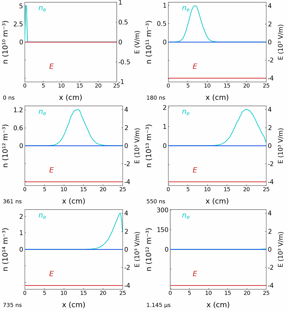
Figure 85 (animation): electron density profile during the transit. The packet leaves the cathode as a narrow pulse and crosses the gap as a travelling wave that becomes more and more asymmetric. Its amplitude grows exponentially by impact ionization, while longitudinal diffusion makes it wider.

Figure 86: the same information as a space-time map of the electron density.

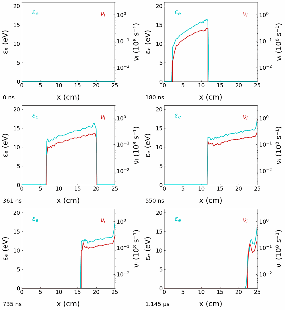
Figure 87 (animation): spatial profiles of the mean electron energy and of the local ionization frequency during the transit. Both increase toward the leading edge of the swarm. The front contains the electrons that move forward fastest, and these electrons are also those that gain the most energy from the field. The front of an avalanche is therefore hotter and ionizes more than its body. This is a kinetic effect: a fluid model with a local-field closure gives a flat energy profile.

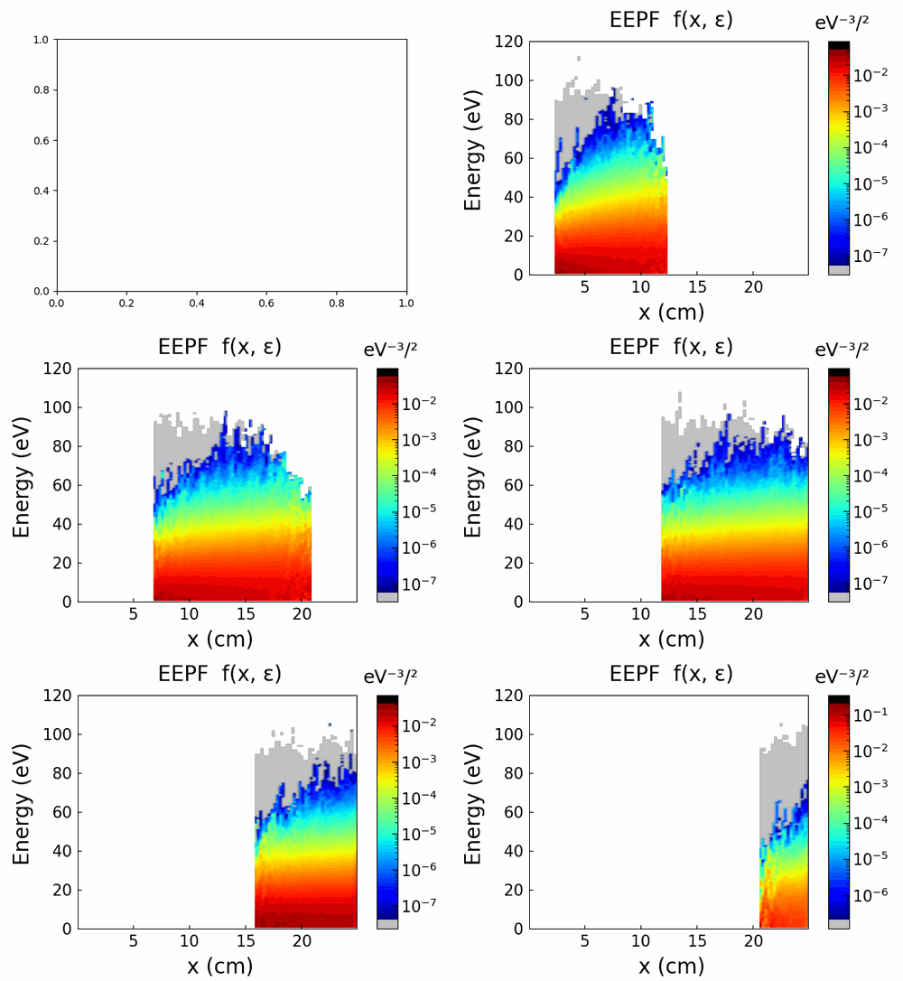
Figure 88 (animation): the electron energy distribution across the swarm. This is the hotter front of Figure 87, seen at the level of the full distribution.

Figure 89: the induced current $I(t)$, on a semi-log scale. There are three regimes. First, an exponential growth while the swarm travels far from the boundaries (a straight line on this plot). Second, a maximum at $t \simeq 0.74$ µs. Third, a sharp collection phase in which the current falls to zero as the anode absorbs the electrons.

Extracting the coefficients from the waveform

This is what an experimentalist has to do. The simulation allows each step to be compared with the known answer.

Ionization frequency. During the flight phase the boundaries play no role and the current grows as $e^{\nu_i t}$. The slope of the straight part (0.30 to 0.40 µs) gives $\nu_i = 1.61\times10^{7}$ s⁻¹, that is $\nu_i/N = 5.00\times10^{-16}$ m³/s. This is within 3 % of the value computed by the swarm mode of the previous sub-section for the same gas at the same reduced field ($5.15\times10^{-16}$ m³/s). The early slope is a reliable measurement.

Drift velocity: the trap of the current peak. It is tempting to read the transit time from the position of the current maximum. This is wrong here, and the error is large. The true drift velocity of this swarm is $v_d = 2.83\times10^{5}$ m/s, so the true transit time is $d/v_d = 0.88$ µs. But the current reaches its maximum at 0.74 µs. The exponential factor $e^{\nu_i t}$ inside the current integral moves the maximum to an earlier time. The peak occurs when the exponential production is exactly balanced by the absorption at the anode, not when the swarm arrives. Reading $v_d = d/t_{peak}$ would overestimate the mobility by 19 %.

Longitudinal diffusion. The classical simple method, which fits the decay of the current with a freely spreading Gaussian, fails for the same reason. The correct model imposes the absorbing boundary $n_e(d,t) = 0$ by the method of images [51-52]. This gives, for the current near the collection phase:

Setting $dI/dt = 0$ at the measured peak time gives one equation for the single unknown $D_L$. With $d = 0.25$ m, $t_{peak} = 0.74$ µs and the values of $v_d$ and $\nu_i$ obtained above, the solution is $D_L \simeq 402$ m²/s, that is $N D_L = 1.295\times10^{25}$ m⁻¹s⁻¹. The code’s own coefficient is $1.298\times10^{25}$: the agreement is 0.3 %.

What this case shows

The waveform contains all three coefficients, but none of them can be read directly when the ionization is strong: the current peak does not mark the transit time, and the decay is not a free Gaussian. With the analytical model that takes the absorbing anode into account, all three coefficients are recovered from one terminal current, exactly as in the laboratory. The ionization frequency is recovered to 3 % and the diffusion coefficient to 0.3 %. The width of the collection phase looks like an abnormally strong diffusion, but it is not. It is the exponential growth that delays the removal of the trailing edge.

III.C. Case 2 The Steady-State Townsend Experiment

The steady-state Townsend (SST) experiment is the oldest and still the most direct way to measure the two coefficients that govern a self-sustained DC discharge. The first Townsend coefficient $\alpha$ is the number of ionizing collisions made by one electron per unit length of drift. The second Townsend coefficient $\gamma$ is the number of electrons released at the cathode per incident ion. Both are obtained from a single, purely electrical measurement: the current through a plane-parallel gap, recorded while the gap length is varied at constant reduced field. This case reproduces this measurement numerically in neon. It then does what no experiment can do. It compares the coefficients obtained from the currents with the coefficients actually used by the code, and shows where the classical analysis fails.

The Method

The apparatus is a plane-parallel gap of length $d$ in a gas at pressure $p$, with a uniform field $E = V/d$. The cathode is illuminated so that it emits a small, constant and independently measured photoelectric current $I_0$. The current is kept low enough that the space charge of the drifting carriers does not perturb the applied field. This is what makes the experiment a swarm experiment and not a discharge experiment. It is also the condition under which $\alpha$ and $\gamma$ are well-defined functions of $E/N$ alone.

Each primary electron produces $e^{\alpha d}-1$ ions on its way to the anode. These ions drift back to the cathode and release $\gamma$ secondary electrons each, which start their own avalanches, and so on. The sum of the geometric series gives the Townsend relation between the collected current and the gap length,

which is the single equation on which the whole method is based. The denominator is zero when $\gamma\left(e^{\alpha d}-1\right)=1$: this is the Townsend breakdown criterion, and an SST measurement must stay well below it [5].

The experimental protocol follows directly. The gap is varied while the applied voltage is varied in proportion, so that $E/N$, and therefore $\alpha$ and $\gamma$ themselves, stay fixed and only $d$ changes. At small $d$ the ion feedback is negligible, the denominator is equal to one, and $\ln(I/I_0)$ is a straight line of slope $\alpha$. At larger $d$ the measured current rises above this straight line. The upward curvature is the signature of $\gamma$: the larger the secondary emission, the earlier the departure from the line. In practice the relation is rewritten as

and $\gamma$ is adjusted until the points fall on a straight line, whose slope is then $-\alpha$. This is essentially the construction introduced by Gosseries [53] and used by Kruithof [54] to produce the reference ionization-coefficient data for the rare gases that are still quoted today. Later measurements in pure neon [55] confirmed and refined them. The same construction is described in the standard textbook treatments of the Townsend regime [45].

Two warnings must be given with the method from the start. First, $\gamma$ is not a property of the gas alone. It combines ion-induced electron emission, emission by fast neutrals and by photons, and gas-phase processes, and it depends strongly on the state of the cathode surface [47]. Second, and this is the subject of the last part of this description, the derivation assumes that $\alpha$ is a local constant everywhere in the gap. In other words, it assumes that the electrons are everywhere in equilibrium with the field. This assumption fails near both electrodes.

The Simulation Setup

The simulation reproduces the experiment as exactly as possible.

Gas: neon at 0.5 Torr and 300 K, i.e. a neutral density of 1.61×10²² m⁻³. Reduced field: $E$ = 2000 V/m in all three cases, i.e. $E/N$ = 124 Td, or $E/p$ = 40 V cm⁻¹ Torr⁻¹. Gaps: $d$ = 3, 5 and 7 cm, with −60, −100 and −140 V applied to the left electrode (the cathode); the anode is grounded. The gap is varied at constant $E/N$, exactly as in the experiment. Primary current: a thermal electron emitter at the cathode, $J_0$ = 10⁻⁵ A m⁻², injecting a flux-weighted Maxwellian at 2 eV. It plays the role of the photoelectric current and is known exactly. Secondary emission: $\gamma$ = 0.30 at the cathode only, secondaries emitted as a 2 eV flux-Maxwellian. This is the number that the analysis must recover. No initial plasma: the gap starts empty and is filled by the injected current alone, so that only the Townsend mechanism is active.

The primary current is deliberately small. At steady state the ion space charge perturbs the potential by less than 0.1 V out of 60 to 140 V. So the field stays uniform to better than a tenth of a percent and the swarm condition is really satisfied.

Accelerating the Calculation: the Lightened Ion

An SST calculation converges on the ion transit time, by far the longest time scale of the problem. At 124 Td neon ions drift at about 10³ m s⁻¹, so crossing 7 cm takes about 80 µs, against 0.2 µs for the electrons. Simulating four or five ion transits with a picosecond time step is too expensive. The ion population is also about two hundred times denser than the electron population, because it is that much slower, so it also dominates the number of macro-particles.

However, the SST steady state does not depend on the ion mass at all. The measurement sees the ion flux returning to the cathode, and continuity fixes this flux entirely from the ionization source,

whatever the ion mobility. In addition, the ion energy distribution is itself invariant under a change of mass. The thermal energy of the target is $kT$ and the energy gained between two collisions is $eE\lambda$. Both are independent of the mass, so only the velocities are rescaled, as $m^{-1/2}$. Dividing the ion mass by a factor $f$ therefore leaves $\Gamma_i(0)$, $n_e(x)$, $\alpha$, the measured current and the ion energy distribution unchanged. At the same time it divides the ion transit time by $\sqrt{f}$, and also the ion density and therefore the number of ion macro-particles.

The three runs use $f$ = 1000, which shortens the ion transit by a factor 31.6 and reduces the number of ion macro-particles by the same factor. A converged steady state is reached in about 8 µs of simulated time instead of 250 µs. The engine implements this as ion_mass_factor in the Advanced → Special panel. The one quantity that must not be lightened is the mass seen by the electrons in their elastic energy loss, $2m_e/M$. Giving the electrons the reduced mass would multiply their cooling rate by $f$, remove the tail of the distribution and destroy $\alpha$. The engine therefore keeps the true gas mass for this term alone. The method is valid only as long as the space charge remains negligible, which is exactly the SST condition. It must not be used with a magnetic field, nor for any time-resolved ion dynamics.

The Measured Currents

At steady state the total current is uniform across the gap and equal to the electron flux collected at the anode. Normalised to the injected primary current, the three simulations give:

Table 1: collected current, ion flux back to the cathode and secondary flux released, for the three gaps, normalised to the injected primary current; last column, the apparent Townsend coefficient.

The third column is the ion flux arriving at the cathode and the fourth is the secondary electron flux that it releases. Their ratio is 0.311, 0.289 and 0.300. This recovers the imposed value of $\gamma$ within the statistical noise. This is an internal check that a real experiment cannot make.

The last column is the apparent Townsend coefficient that would be read if the ion feedback were ignored. It is not constant: it increases from 13.9 to 27.7 m⁻¹ as the gap becomes wider. This increase is the raw signal used by the method.

Extracting the Two Coefficients

Applying the classical construction to these three points gives an instructive failure. For any assumed $\gamma\geq 0$, the value of $\alpha$ deduced from each gap separately still increases with $d$. For $\gamma$ = 0.3 one obtains 10.2, 13.3 and 15.4 m⁻¹, and no choice of $\gamma$ makes the three values agree. The measured curvature is stronger than the ion feedback alone can produce. In the language of the experiment, the three points cannot be put on a straight line.

The missing element is the finite distance that the electrons need, after leaving the cathode, before they ionize at all. Replacing the geometrical gap by an effective gap $d-d_0$ restores consistency. With $\gamma$ kept at its true value of 0.30, the three points give $\alpha$ = 18.8 m⁻¹ and $d_0$ = 13.9 mm. The residual scatter between the three gaps is 1.8 %. If instead $\alpha$, $\gamma$ and $d_0$ are all left free, the fit is formally better (0.2 %) but gives $\gamma$ = 0.61 and $\alpha$ = 13.0 m⁻¹. The secondary emission coefficient is then overestimated by a factor of two and $\alpha$ is underestimated by a third. Three gap lengths simply do not contain enough information to separate three strongly correlated parameters. This is the practical reason why real SST campaigns use a dozen gap values and several pressures, and restrict the analysis to gaps much larger than $d_0$.

For neon at $E/N$ = 124 Td the hydrodynamic value of the ionization coefficient is $\alpha_{sw}$ = 24.0 m⁻¹. This value is computed with the same cross sections by the swarm module of JC-PIC running in its spatial-growth (SST) mode [38]. This is $\alpha/N$ = 1.49×10⁻²¹ m² or $\alpha/p$ = 0.48 cm⁻¹ Torr⁻¹ at $E/p$ = 40 V cm⁻¹ Torr⁻¹. The value recovered from the currents, 18.8 m⁻¹, is 22 % below it. This difference is not numerical noise. It is physics, and the profiles show where it comes from.

The Non-Equilibrium Regions

Figure 90: Spatial profile of the mean electron energy and ionization frequency across the 5 cm gap at steady state. Electrons enter at 2 eV and need about one centimetre to reach the plateau at 13.5 eV. The rise in front of the anode is the flux-weighted signature of the absorbing boundary. Ionization is absent over the first centimetre (the cathode relaxation zone), then reaches a plateau, and decreases again over the last few millimetres in front of the anode.

The mean electron energy is far from uniform. Electrons are emitted at the cathode with a few eV. They must gain energy from the field before they can excite (16.6 eV) or ionize (21.6 eV) a neon atom. Neon has no Ramsauer minimum and a nearly constant elastic cross section, so the momentum-transfer mean free path is only 2.1 mm. The electrons therefore gain energy by a random walk and not by ballistic acceleration, and the rise in energy takes about a centimetre. The plateau value, 13.5 eV, agrees within 3 % with the 13.1 eV given by the swarm calculation at the same $E/N$. The bulk of the gap is therefore close to energy equilibrium.

The ionization profile makes the consequence explicit. Over the first ten to twelve millimetres the ionization rate is almost zero. This is the cathode relaxation zone, and it is what the effective-gap correction $d_0$ represented. Beyond this zone, the local coefficient $\alpha_{loc}(x)=S_{iz}(x)/\Gamma_e(x)$ is between 18.6 and 19.3 m⁻¹. This is exactly the value returned by the current analysis, which confirms that the analysis measures the plateau and not some average. Finally, over the last few millimetres before the anode the ionization decreases again. Electrons that would have been scattered back into the gap are absorbed instead, so the high-energy part of the distribution is depleted there. This is the anode layer.

This still leaves the residual 22 % between the plateau value and the equilibrium swarm value. The gap is only about one and a half e-folding lengths long. A large fraction of the electron population at any instant is “young”: either newly injected at the cathode, or newly created by ionization at low energy. The tail of the distribution above the 21.6 eV threshold is what $\alpha$ measures. This tail is therefore never as fully developed as in an infinite uniform swarm, even where the mean energy has already relaxed. The mean energy reaches equilibrium much faster than the ionizing tail.

What This Case Shows

The simulation reproduces the SST measurement correctly. The currents increase with the gap exactly as Townsend’s relation predicts. The ion flux to the cathode releases secondaries at the imposed rate. The coefficient extracted from the currents is equal to the local coefficient measured directly inside the gap. It also shows the two systematic difficulties that every real SST measurement has to face, and which are invisible to an experiment that sees only the terminal current. The cathode relaxation zone biases $\alpha$ downwards unless it is explicitly subtracted, and it is not small here: 14 mm against a shortest gap of 30 mm. And the fitted parameters are strongly correlated, so a small number of gap lengths can return a $\gamma$ twice the true one while fitting the data almost perfectly.

The remedies are those adopted by the experimentalists long ago. Work at pressure–distance products large enough that the relaxation zone is a small fraction of the gap. Use many gap lengths. Treat $\gamma$ as a surface-dependent parameter and not as a property of the gas. Repeating this case at 1 Torr with the same $E/N$, that is, at twice the value of $pd$, halves the relaxation zone relative to the gap. It is a useful exercise to see the extraction improve.

III.C. Case 3 The Franck-Hertz Experiment

This experiment was performed in 1914 by James Franck and Gustav Hertz. It is one of the founding experiments of quantum physics [56]. Franck and Hertz sent electrons of controlled energy through a low-pressure vapour and measured the collected current. They found that the current decreased sharply at regular intervals of the accelerating voltage, 4.9 V in mercury. This showed that an atom can only absorb energy in discrete amounts. They first interpreted the 4.9 V as an ionization potential. The following year, Bohr identified it as the excitation energy of the first quantum level. The result thus became the first direct confirmation of his model [57]. The two experimenters received the 1925 Nobel Prize in Physics for this work.

From the point of view of modern gaseous electronics, however, the Franck-Hertz tube is not a beam experiment [58]. It is a steady-state Townsend discharge operated well below the ionization threshold, in a strongly non-hydrodynamic regime. The electrons are a swarm, not a beam. They scatter elastically hundreds of times between two inelastic events. The periodic structure that made the experiment famous is the spatial relaxation oscillation of their energy distribution. A kinetic simulation can show this directly. This is the subject of this case.

The Experiment

The apparatus is a drift tube, planar or cylindrical, filled with a low-pressure vapour or gas. The original work used mercury; the version used in teaching laboratories today uses neon at a few mbar. The tube has three electrodes. A thermionic cathode emits the electrons. An accelerating grid held at a variable potential $V_{acc}$ creates a nearly uniform field across the drift space. Finally, a collector anode is placed just beyond the grid. It is held at a small retarding potential $V_{ret}$ of one or two volts. It therefore collects only the electrons whose longitudinal kinetic energy is still larger than the barrier,

When $V_{acc}$ is increased, the collected current $I_A$ increases, then decreases sharply, then increases again, and so on, with a regular period. The decrease occurs each time the electrons have gained just enough energy, when they reach the grid, to lose all of it in an inelastic collision. They are then unable to pass the retarding barrier. In neon the period is close to 18.7 V. The tube also shows directly what the current measurement only suggests: a set of orange luminous layers, parallel to the electrodes, one per period. These layers move and multiply when the voltage is increased. Each layer marks a region where the electrons have enough energy to excite the gas.

Why 18.7 V and not 16.6 eV

The textbook version of the experiment assumes a monoenergetic, unidirectional beam that excites the atom as soon as it reaches the threshold. Neither assumption is correct, and the difference can be measured. Neon does not have a single first excited level but a group of them. The electron-impact thresholds that matter here are:

Table 1: the electron-impact thresholds of neon that matter for the Franck-Hertz experiment.

Three effects make the observed period larger than the lowest threshold. The excitation cross section increases slowly from threshold. So an electron that has just passed 16.6 eV usually continues to accelerate over some distance before it actually collides. Elastic collisions with the neon atoms transfer almost no energy, because of the mass ratio, but they randomize the direction completely. They therefore spread the electron energy distribution, so that “the” energy at a given position is only a mean. When the energy increases beyond 18.4 eV, the $3p$ group of levels becomes accessible, with cross sections large enough to dominate the losses. The measured period is therefore a weighted average over all open channels. It is close to 18.7 V rather than 16.6 V. One of the results below is that the simulation reproduces this number from the cross sections alone.

The light needs a separate explanation. The $3s$ states decay to the ground state in the vacuum ultraviolet, which is invisible. The two metastable states do not decay radiatively at all. The orange-red bands that are actually seen come from the cascade $3p \rightarrow 3s$, whose lines lie between about 585 and 730 nm. The luminous layers are therefore a map of the $3p$ excitation rate. This rate is itself a map of the regions where the electrons are energetic.

The Simulation: a Different Cut Through the Same Physics

The simulation deliberately does not reproduce the voltage sweep. The applied voltage is fixed, and the spatial structure of the electron swarm along the gap is examined at steady state. The two views are equivalent. In a uniform field the energy gained by an electron is $eEx$. So scanning the grid position at fixed field and scanning the field at fixed grid position probe the same variable. Reading the structure in $x$ gives much more information: instead of one number per run, one obtains the whole distribution function, at every position, at once.

The run is done in Laplace mode (no_poisson = 1): the field is imposed and uniform, Poisson’s equation is not solved, and the ions are neither pushed nor collided. This is valid here because the current is very small and the space charge is negligible. It also makes the calculation cheap. It also means that the case describes only the electron kinetics. It says nothing about the ion space charge, which does play a role in a real tube at higher currents.

Gas: neon at 1 Torr and 300 K, i.e. a neutral density of 3.22×10²² m⁻³. Gap and field: 40 cm with −200 V applied, i.e. $E$ = 5 V/cm, exactly uniform, or $E/N$ = 15.5 Td. Electrons gain 5 eV per centimetre of drift. Cathode source: a monoenergetic 1 eV electron beam injected at $x$ = 0 with a current density of 10⁻³ A m⁻². It plays the role of the thermionic emission. Diagnostics: the gap is long enough to contain about ten Franck-Hertz periods. The run reaches steady state after about 3 µs (the electron transit time), and the profiles are averaged from 10 to 15 µs.

The collisions do not conserve the number of electrons exactly, because ionization is weak but not zero at these energies. The case is therefore a Townsend discharge on a small scale. The ionization mean free path, 18 cm, is comparable to the gap, so the multiplication remains small.

The Franck-Hertz Oscillation in Space

Figure 91: Mean electron energy along the gap. The swarm enters at 1 eV, is accelerated to a first maximum of 15.1 eV at x = 3.2 cm, decreases to 4.8 eV, and repeats. The oscillation is damped over about ten periods towards the equilibrium swarm value.

This is the Franck-Hertz effect in its simplest form. The electrons enter with a low energy and gain 5 eV per centimetre. Around 3 cm, the fastest of them start to cross the neon excitation thresholds. The inelastic collisions then remove 16 to 20 eV in one step, and the mean energy decreases sharply. The cycle starts again and repeats along the tube.

Measured on the first seven maxima, the spatial period is $\Lambda$ = 3.72 cm. Multiplied by the field, this gives an energy of

This value is to be compared with the 18.7 V period measured in real neon Franck-Hertz tubes [59], and with the 16.62 eV lowest threshold of neon. The simulation therefore reproduces the experimental period. It also shows that the excess over the lowest atomic threshold is a purely kinetic effect, not an atomic one. It comes from the shape of the cross sections and from the spread of the distribution. Both are included in the calculation, and neither is included in the textbook picture.

The oscillation is also damped. The maxima decrease from 15.1 to about 9 eV and the minima increase from 4.8 to about 8.5 eV. By 30 cm the contrast has almost disappeared and the mean energy remains constant at 8.3 eV. This plateau is the hydrodynamic equilibrium of the swarm [5]. The swarm module of JC-PIC, run at the same $E/N$ with the same cross sections, gives 8.07 eV, which is an agreement within 3 %. In the real experiment the same damping is visible as the progressive weakening of the current oscillations at high $V_{acc}$.

Where the Damping Comes From

Figure 92: Electron distribution function $f_e(x,\varepsilon)$. Each straight branch is one generation of electrons accelerating freely at 5 eV/cm. Each branch is cut near 20 eV by the inelastic collisions, which return the electrons to low energy and start the next branch. Successive generations become broader. Beyond about 20 cm, the population fills the whole 0–20 eV band uniformly.

The energy-resolved distribution shows the mechanism directly. The first branch is a narrow line that starts from 1 eV at the cathode and rises with exactly the slope $eE$ = 5 eV/cm. It is the injected beam, still monoenergetic. It is cut off around 20 eV, where the inelastic cross sections have become large. The electrons that have collided reappear at the bottom of the energy axis and form a second branch. This branch is already visibly wider, because the electrons did not all collide at the same energy and did not all lose the same amount. The excitation thresholds are spread over 16.6 to 20.6 eV. Each generation is broader than the previous one. This is phase mixing. After about ten cycles the memory of the injection is completely lost, the branches overlap, and the distribution becomes the stationary distribution of an infinite swarm in a uniform field. The sharp upper edge near 20 eV remains, because it is set by the thresholds and not by the history.

Figure 93: Electron distribution in phase space, $f_e(x,v_x)$. The nested arcs are the same generations seen in velocity. Each arc is the parabola $v_x^2 = v_0^2 + 2(eE/m)x$ of free acceleration, cut by the inelastic collisions. The distribution is symmetric in $\pm v_x$: this is a swarm, not a beam.

The phase-space view adds the point that the textbook picture misses most. The distribution is symmetric in $v_x$ everywhere, including inside the first arc: as many electrons move backwards as forwards. The elastic mean free path is only 1.3 mm, against a period of 3.7 cm. An electron is therefore scattered several hundred times per cycle, and its actual path length is about 24 times its net displacement. It travels about one metre to advance 3.7 cm. The periodic quantity in space is not a trajectory but the local energy balance. The Franck-Hertz period is set by the potential drop needed to reach the threshold, and by nothing else. No mean free path enters it. This is why $\Lambda$ is proportional to $1/E$ and is independent of pressure.

The Luminous Layers

Figure 94: Excitation frequency of the neon 2P group of levels ($2p^5 3p$, threshold 18.72 eV), left logarithmic axis, together with the mean electron energy, right linear axis. These are the states whose cascade to $3s$ produces the visible light. The excitation rate is exactly zero over the first 3.5 cm. It then has one maximum per Franck-Hertz period, with a contrast of nearly three decades in the first cycle. Each emission maximum is located about 1.1 cm downstream of the corresponding energy maximum.

This is the quantity that the eye sees in the tube. The channel plotted is the one that actually radiates. The $3s$ states reached at 16.6 eV are either metastable or decay in the vacuum ultraviolet. The $2p^5 3p$ group of levels at 18.72 eV cascades down to $3s$ in the orange-red. The rate is zero until the electrons have gained the threshold energy. This takes 3.74 cm at 5 eV/cm, and the first layer indeed appears at 4.0 cm. In the first cycle the ratio between maximum and minimum reaches three orders of magnitude. This is why the layers appear as sharp bright bands on a black background rather than as a weak modulation. Further along the tube the ratio decreases to a factor of two or three. This is the same phase mixing that flattens Figure 91. The period read on this channel, 3.73 cm, corresponds to 18.7 eV. This is the experimental value, obtained a second time, and now on the very quantity that is observed.

The two curves are not in phase, and the shift is systematic. Over the first seven cycles each excitation maximum is located strictly between a maximum of the mean energy and the following minimum. On average it is 1.11 cm behind the energy maximum, which is 0.30 of a period, or 5.6 V of potential drop. The reason is that the two quantities do not sample the same part of the distribution. The mean energy is a bulk average, dominated by the many slow electrons. The excitation rate is a threshold quantity, produced only by the tail above 18.7 eV. The mean energy stops increasing exactly when the inelastic loss rate has become large enough to balance the power taken from the field. This happens on the rising side of the excitation rate, not at its maximum. The rate continues to increase while the mean energy is already decreasing. It reaches its maximum only when the tail has been emptied. The practical consequence for the experiment is that a bright layer is not centred where the electrons have the highest energy. It is located about a third of a period further towards the anode.

One limitation of the comparison with a real tube: the simulation contains only direct excitation from the ground state. In a working neon tube the $2p$ states are also populated in two steps from the accumulated $3s$ metastables. This channel increases with pressure and current, and it would partly fill the deep minima.

The Same Resonance in a Self-Consistent Field

The structure seen here is the response of the electron energy distribution to a field that is given. The period is the length an electron needs to reach the first inelastic threshold, and nothing in the plasma reacts to it. When the field is instead produced by the plasma itself, the same resonance organises the discharge by itself, and the layers start to move. This is the striation of a positive column. It is treated in Striations in a DC positive column plasma in the Positive Column chapter, and analysed in detail in [41].

The mechanism is clearly the same: periodic layers of excitation, separated by the potential drop needed to reach the neon thresholds. Two differences deserve a comparison. First, in the positive column the field is the sum of the applied field and the space-charge field, so the potential jump adjusts itself. The drop measured across one striation there is 10 to 12 V, a fraction of the excitation threshold, against the full 18.7 V imposed here. The striation length, about 2 cm at 6 V/cm, follows that smaller drop. Second, and more fundamentally, the positive-column structure acts back on the ionization that sustains the plasma, so it is unstable. The layers grow from a uniform initial state and then propagate towards the cathode. The Franck-Hertz layers, on the contrary, are strictly stationary. They are simply imposed on the swarm by the boundary condition at the cathode. In this sense, the Franck-Hertz tube is the forced and stationary version of the striation.

What to Take Away

The simulation reproduces the two classical observables of the Franck-Hertz experiment, the periodicity and the luminous layers, from nothing but the electron-neon cross sections and a uniform field. It obtains the correct period: 18.6 eV against 18.7 V measured. In doing so, it makes explicit what the historical interpretation compresses into a single number. The period is not the atomic excitation energy. It is that energy convolved with the shape of the cross sections and with the width of the electron energy distribution. This is why it is two volts larger than the lowest threshold. The electrons are not a beam but a swarm, scattered hundreds of times per cycle. The damping of the oscillations is not explained at all by the textbook picture. It is the phase mixing of successive electron generations, which relax towards the ordinary hydrodynamic equilibrium of a swarm in a uniform field. This is the state described by the swarm parameters of the previous cases in this chapter.

IV Electron Emission from Cathode

The emission of electrons from a cathode gives the boundary condition for a large class of devices: vacuum tubes, electron guns, gas discharges and electric thrusters. The current that a cathode can deliver is not limited by the emitter itself. It is limited by the space charge of the electrons that are already in flight [60]. When the number of emitted electrons increases, they reduce the potential in front of the cathode and reduce the emission. This chapter uses Particle-In-Cell (PIC) simulations to study this physics with a kinetic model, in two complementary parts: a collisionless Vacuum Diode and a collisional Thermionic Discharge.

The Vacuum Diode

The first part studies the space-charge limitation alone, in a pure vacuum gap. It is based on the classical Child-Langmuir law [61-62]. This law gives the maximum current density that a cathode can send across a gap, for a given voltage and a given gap length. It applies when the electrons are emitted with a negligible initial energy. The law can also be extended to a finite injection energy [63]. The Child-Langmuir case runs a beam at the space-charge-limited current, then above it, and shows the potential minimum that appears. The Virtual Cathode Oscillations case increases the injected current above the limit. A potential minimum, called a virtual cathode, forms near the emitter. Above a second threshold this minimum starts to oscillate [64]. Finally, the Thermionic Emission case replaces the mono-energetic beam with a half-Maxwellian flux from a hot cathode. The low-energy electrons that cannot cross the potential minimum are reflected back to the cathode. This reflection stabilises the virtual cathode and suppresses the oscillations.

The Thermionic Discharge

In the second part the emitted electrons ionise a low-pressure background gas. They produce a self-sustaining plasma. The structure of this plasma is fixed by the electron beam, the neutral gas and the self-consistent ions together. The emission current follows the Richardson-Dushman law, and the steady state corresponds to one of several well-known operating regimes [65]. The Temperature-Limited Current (TLM) case works at a voltage much above the ionisation threshold. It produces a quasi-neutral plasma with an ion-rich cathode sheath and no virtual cathode. The TLM with Beam-Plasma Instability case shows that, at high emission current and low pressure, this mode can become unstable and give beam-plasma oscillations. The Anode Glow Mode (AGM) case shows a different low-current regime [65], in which an inverse cathode sheath forms and the ionisation is concentrated in a thin layer near the anode. Lastly, the AGM Self-Oscillations case shows that this mode is unstable by nature. It gives the low-frequency relaxation oscillations and the period-doubling route to chaos that are typical of thermionic discharges [66].

These cases are pre-configured. They can be run, and the phase space and the potential profiles can be inspected. The space-charge limitation, the formation of the virtual cathode and the self-organisation of the discharge are then observed directly as results of the kinetics. Simple circuit models or fluid models cannot describe these phenomena.

IV.A Vacuum Diode: Space-Charge-Limited Emission

A vacuum diode is the simplest device in which a cathode emits electrons across a gap toward an anode at a positive voltage. It shows one essential point of physics. The current that a cathode can deliver is not limited by the emitter itself. It is limited by the space charge of the electrons that are already moving across the gap [60].

The Physical Mechanism

When electrons leave the cathode, they bring negative charge into the gap and they lower the local potential. If the emission is strong enough, this accumulation of charge reduces the electric field at the cathode surface to zero. Any additional electron then finds no accelerating field and is turned back. The diode therefore limits itself to a maximum current, the space-charge-limited current, also called the Child-Langmuir current.

The Child-Langmuir Law

Consider a plane gap of width $d$, with the cathode at $x = 0$ and a voltage $V$ applied across it. The electrons are emitted with a negligible initial energy. Three relations are enough to solve the problem. The conservation of energy for an electron that has crossed the potential $\phi(x)$ gives its velocity,

the steady current density is the same everywhere in the gap,

and Poisson’s equation links the potential to the electron charge density,

By eliminating $n$ and $v$, and by imposing the space-charge-limited condition $d\phi/dx = 0$ at the cathode, one obtains the Child-Langmuir law [61-62]:

The current increases as $V^{3/2}$, and not linearly as in an ohmic conductor. It decreases as $1/d^2$. This behaviour shows that the current is controlled by the space charge and is not limited by the emitter.

Beyond the Cold Limit

This result assumes that the electrons start at rest. They can also be injected with a finite energy: the directed energy of a beam, or the thermal spread of a hot cathode. The limiting current is then modified, and the potential can have a true minimum in front of the cathode, and not only a point where the field is zero. This minimum is a virtual cathode [63]. The two following cases study this regime.

The Cases in This Part

The Child-Langmuir case runs a beam first at the zero-field current, then above $J_{CL}$. It checks the density and potential profiles and the $V^{3/2}$ scaling. The Virtual Cathode Oscillations case injects a beam above the limit. A virtual cathode is formed and, above a second threshold, it starts to oscillate [64]. The Thermionic Emission case replaces the mono-energetic beam by a half-Maxwellian flux from a hot cathode. In this case the low-energy electrons reflected by the dip of the potential stabilise the virtual cathode and suppress the oscillations.

IV.A. Case 1 Child Langmuir Law

We consider a planar vacuum diode: a cathode at x=0 held at a voltage -V, and a grounded anode at x=d. Electrons are injected at the cathode and accelerated in the gap. The Child-Langmuir Law [61-62] gives the maximum current density that can flow through a vacuum diode under space-charge-limited conditions, when the electrons leave the cathode with an energy that is negligible compared to the applied voltage.

Physics

At steady state the current density $J$ is limited by the geometry and the voltage of the system. The law states that the current density is proportional to the voltage raised to the power of 3/2 and inversely proportional to the square of the distance:

For electrons emitted with a negligible energy, this current is the current for which the electric field at the cathode is zero, $E(0)=0$, and it is the maximum current that can be transmitted. These two conditions coincide because the smallest negative dip in the potential would reflect electrons that arrive with zero energy. If more current than the Child Langmuir current is injected, a negative space-charge barrier forms in front of the cathode and sends the excess back: the diode limits itself. This is the defining property of the Child-Langmuir regime [60]. The Child Langmuir law is derived by combining Poisson’s equation with $E(0)=0$, conservation of energy for the electrons, and current continuity.

If the electrons are injected with a directed energy W₀ (in eV), the space-charge relation generalizes to:

It reduces to the Child Langmuir relation for W₀=0. This formula is the condition of zero field at the cathode (E(0)=0) with a non-zero injection energy. It is the current at which a potential minimum just begins to form at the cathode. It is not the maximum current that a beam of energy W₀ can carry. With a finite injection energy, “field zero at the cathode” and “maximum transmittable current” no longer coincide: - For J < J(E0=0): the field is accelerating everywhere, the potential is monotonic, there is no dip. - At J = J(E0=0): the potential minimum appears, with a depth still equal to zero. - For J > J(E0=0): a dip forms and becomes deeper, but electrons of energy W₀ are reflected only when the dip reaches -W₀. The true current limit (onset of reflection and formation of a virtual cathode) is therefore higher than this formula. See the Virtual Cathode Oscillations case.

Conditions of the simulation

In this example, monoenergetic electrons are emitted from the cathode with an energy W₀. Gas pressure 0 Cathode voltage -V=-50 V Gap length d=2 cm Beam electron energy W₀= 5 eV Emitted electron current density 4.27 A/m² (corresponding to E(0)=0) Initial Conditions Plasma density 0 Number of grid points 256 Time step 10⁻¹² s Number of electrons 30000 (this number in fact fixes the number of electrons emitted per dt in the simulation, for the given current density)

Results

According to the formula above, the field should be zero at the cathode for a current density Jₑ₀=4.27 A/m² This can be checked in the simulation (see Figs. 95 and 96).

Figure 95: Spatial profiles of electron density and electric field (W₀=5 eV, Jₑ₀=4.27 A/m²)

Figure 96: Spatial profile of electron density and electric potential (W₀=5 eV, Jₑ₀=4.27 A/m²)

The simulation can be run with a larger current density. A virtual cathode (potential minimum) then forms inside the gap, close to the cathode (see Fig. 97, where Jₑ₀=5.2 A/m²). In the example of Fig. 97, the minimum potential is about 1.5 V below the cathode potential. A maximum of the electron density appears at the position of the virtual cathode. If the current is increased above a given limit (around 5.3 A/m² in this example), oscillations of the virtual cathode appear (second example in this section). These oscillations appear when the potential drop in the virtual cathode becomes larger than W₀.

Figure 97: Spatial profile of electron density and electric potential (W₀=5 eV, Jₑ₀=5.2 A/m²). The potential is plotted in the interval [-52 V, -50 V].

IV.A. Case 2 Thermionic Emission

In this example the electron emission is thermal (Maxwellian emission). The electrons are emitted from the cathode with a half-Maxwellian flux distribution at the temperature Tₑ (in eV). An optional shift vₓ₀ in velocity can also be given.

Physics

The flux of emitted electrons is given by:

The flux is integrated over a half space in velocity (vₓ>0). For this reason the exact drift velocity of the emitted electrons is not vₓ₀. It is larger than vₓ₀, because the emitted electrons have a finite temperature. For a purely thermionic emission vₓ₀=0. The mean axial velocity (flux-weighted) of the emitted electrons is then:

with $v_{th} = \sqrt{\frac{e\,T_e}{m_e}}$

The flux-weighted mean axial energy of the emitted electrons is Tₑ and their mean total energy is 2 Tₑ.

The phase space (x,vₓ) of the electrons is shown in Fig. 99 below. The space-charge limitation appears because a part of the emitted electrons return to the cathode [62]. The reason is a minimum of the plasma potential close to the cathode (the virtual cathode, see Fig. 98 below). This potential minimum reflects the electrons that are emitted with an axial energy smaller than this potential drop. Langmuir made a detailed study of this regime [63].

The regime of a thermionic vacuum diode is in general stable (no oscillations). For a monoenergetic beam of emitted electrons, instabilities can appear above a given injected current density. These are the virtual cathode oscillations, described in the Virtual Cathode Oscillations case of this section.

Conditions of the simulation

Gap length d=2 cm Cathode voltage V=-50 V Current density of emitted electrons: Jₑ₀=50 A/m² Temperature of emitted electrons Te=3 eV Shift in velocity of emitted electrons vₓ₀=1.33 10⁶ m/s (5 eV)

Results

Figure 98: Spatial profile of electron density and potential.

Figure 99: Electron phase space (x,vₓ)

IV.A. Case 3 Thermionic Emission Test Case

This test verifies the code JC-PIC against an exact kinetic solution for collisionless, space-charge-limited electron flow in a plane diode, following Turner [67]. It is the thermal (Maxwellian-emission) version of the classical Child-Langmuir problem. Instead of a cold mono-energetic beam, a Maxwellian flux of electrons is emitted from one wall, as in the previous subsection “Thermionic Emission”. Because the flow is collisionless, the governing equations are the Vlasov-Poisson system, for which an exact solution is known [1, and references therein, 2-4]. The simulation must converge to this exact solution when the time step, the cell size and the number of particles per cell are refined. This makes it a demanding code-verification benchmark.

Physics

Two grounded walls bound the gap, with the potential held at zero on both, $\phi(0)=\phi(L)=0$. A prescribed flux of electrons with a Maxwellian velocity distribution is emitted from the left wall. Any electron that crosses either wall again is absorbed. The electrons in the gap carry a negative space charge, so the potential becomes negative and develops a minimum $\phi_m$ (a potential well, or virtual cathode). This well reflects the slower electrons back to the emitter and transmits only the faster ones [63]. The current crossing the diode is therefore limited by its own space charge.

The steady-state speed distribution for particles of mass $m$ and charge $q$ can be written as [67]

where $n_0$ is the electron density next to the emitting boundary and $v_t$ the thermal speed,

Integration over velocity gives the density, which obeys a Boltzmann relation,

so the density decreases monotonically from $n_0$ at the emitter as the potential becomes more negative. The current density transmitted through the diode is the first moment of the distribution,

with $\phi_m$ the (most negative) potential of the well and $\Phi_m$ its dimensionless value,

The current is thus controlled by the single dimensionless parameter $\Phi_m$. This parameter is itself fixed by the normalized system length, the gap measured in Debye lengths,

The relationship $\Phi_m(\Lambda)$ is obtained from a quadrature [67] (Turner’s Fig. 103).

A useful way to read the result: a Maxwellian reservoir at density $n_0$ emits a half-Maxwellian flux $\Gamma$, i.e. an emitted current density $q\Gamma$. The transmitted current $J_0$ is this emitted flux reduced by the barrier factor $e^{-\Phi_m}$:

Only a small fraction of the emitted electrons pass the well and reach the anode. The others are reflected and reabsorbed at the emitter.

Conditions of the simulation

Following Turner [67] we set $\Lambda = 20$, which gives $\Phi_m = 2.398$. With

• $T_0 = 10$ eV (temperature of the injected electrons)
• $n_0 = 10^{16}$ m⁻³ (electron density at the emitter)
• $q = -e$, $m$ = electron mass

the derived quantities are

• thermal speed $v_t=\sqrt{2eT_0/m} = 1.88\times10^{6}$ m/s
• Debye length $\lambda_D=\sqrt{\varepsilon_0 T_0/e\,n_0} = 0.235$ mm
• gap length $L=\Lambda\,\lambda_D = 4.70\times10^{-3}$ m
• potential minimum $\phi_m=-\Phi_m\,T_0 = -24.0$ V
• emitted current density $q\,n_0 v_t/(2\sqrt{\pi}) = 847$ A/m², the value imposed at the emitter, not the transmitted current
• transmitted current density $J_0 = 847\,e^{-\Phi_m} =$ 77 A/m²

Gas pressure 0 (collisionless) Both walls grounded (0 V) and fully absorbing (no secondary emission, no ions) Electron injection at the left wall: thermal-source mode (flux-weighted Maxwellian, $v_x$ sampled $\propto v\,e^{-v^2/v_t^2}$), $T_0 = 10$ eV, $J = 847$ A/m²

Initial Conditions Plasma density 0 (the gap is filled self-consistently by the emitted flux) Cathode and anode at 0 V

Numerical parameters The numerical error is quadratic in each of the three numerical parameters (time step, cell size and particles per cell), so convergence is verified by refining all three together [67]. A representative base set is $\omega_p\Delta t = 0.8$ ($\Delta t \approx 1.4\times10^{-10}$ s), about 30 cells across the gap and about 4 particles per cell, which are then refined. The transmitted-current diagnostic in particular needs a small $\Delta t$ and a high particle count to converge. Near the emitter the net current is the small difference of two large opposing fluxes (≈ 847 A/m² emitted against ≈ 770 A/m² reflected), so it is statistically noisy until the particle count is high.

Results

At convergence the simulation reproduces the exact solution: the potential well, the Boltzmann density profile and the transmitted current $J_0$.

Figure 100: Electron density (left axis) and electric potential (right axis). The potential decreases from 0 at the emitter to a minimum $\phi_m \approx -24$ V near $x/L \approx 0.4$ (the space-charge well), then increases again toward 0 at the grounded anode, consistent with $\Phi_m = 2.398$ ($\phi_m = -\Phi_m T_0$). The electron density is highest at the emitter and decreases steeply into the gap, following the Boltzmann relation $n(x)=n_0\,e^{-\Phi(x)}$. With flux injection the emitter density is a few percent below $n_0$, because the fastest emitted electrons are transmitted and never return, which slightly truncates the returning part of the distribution.

Figure 101: magnitude of the discharge current against time. It reaches a constant value of 79 A/m², within 3 % of the exact value 77 A/m² $= J_0 = q\,n_0 v_t/(2\sqrt{\pi})\,e^{-\Phi_m}$. The gap-averaged “total current” is a noisier estimator here, because it is the small net value of the large emitted and reflected fluxes near the cathode. The clean, physically meaningful value is the current collected at the anode.

Figure 102: Electron phase space ($v_x$ versus $x$). Electrons are emitted at $x=0$ with $v_x>0$ drawn from the flux-weighted Maxwellian, and they decelerate as they move up the space-charge well. Low-energy electrons reach a turning point and go back toward the emitter (the reflected branch at $v_x<0$). The high-energy tail ($\frac{1}{2}mv_x^2 > e|\phi_m|$) crosses the well and is collected at the anode. The envelope of the turning points maps the potential well. The dense reflected population near the emitter is what builds the negative space charge.

IV.A. Case 4 Virtual Cathode Oscillations

This case shows what happens when a beam is injected into a vacuum gap with a current above the space-charge limit. A virtual cathode forms, and above a second threshold it oscillates.

Conditions of oscillations

For a beam of injection energy W₀ there are two characteristic currents: - $J(E(0)=0)$ - the Child-Langmuir value with initial energy. At this current the field at the cathode just reaches zero and a potential minimum begins to form :

• $J_{max}$ - the true transmission limit. It is reached when the potential minimum becomes as deep as $-W_0$, that is, when electrons of energy W₀ are finally reflected. Therefore, an injected current between J(E0=0) and $J_{max}$ gives a stable solution with a small potential dip but no reflection. The full beam is transmitted. (For $W_0=0$ the two currents are equal, and any excess current is reflected immediately.)

Physics of the oscillations

When the injected current is larger than Jₘₐₓ, the space charge creates a potential minimum below -W₀. Part of the beam is then reflected. This reflection point is the virtual cathode. Just above the threshold the virtual cathode is stationary. Further above the threshold, the feedback between injected and reflected electrons becomes coherent (the transit times and turning points become aligned). The virtual cathode then begins to oscillate (Bursian or vircator instability). This produces a strong oscillation of the field energy and of the transmitted current.

A cold beam oscillates most strongly. An energy spread (a beam temperature Te) spreads the transit times and the turning points. This destroys the coherence of the feedback (phase mixing) and damps the oscillation above some value of Tₑ. If the distribution of the emitted electrons is a half-Maxwellian (thermionic emission — see the Thermionic Emission case), a virtual cathode may form for current densities above a given limit, but the oscillations are damped.

Applications

This mechanism is the basic principle of the high-power microwave (HPM) generators called Vircators, Virtual Cathode Oscillators [64], [68]. Traditional microwave tubes, such as magnetrons or klystrons, need an external magnetic field to focus the electron beam. A vircator does not need one, so it is light and compact. It can produce gigawatt-level electromagnetic pulses with a simple mechanical design. Practical vircators usually use a gridded or foil anode, so their geometry is more complex than this 1D model. They also operate at very high power and with relativistic electrons. However, the fundamental physics of the oscillating space-charge barrier remains similar.

Conditions of the simulation

The current, beam energy and voltage in this simulation are much smaller than in real devices! (In real devices, the electrons are relativistic.) The aim is only to illustrate the concept of virtual cathode oscillations. Similar particle simulations at low current and low energy are discussed in the book of A. Piel [69], page 253 (“Virtual Cathode of a Thermal Emitter”). Gap length 2 cm Applied voltage 50 V Beam current density 50 A/m² Beam energy 20 eV In these conditions $J(E(0)=0)$ is 6.81 A/m², and $J_{max}$ is between 12 and 13 A/m².

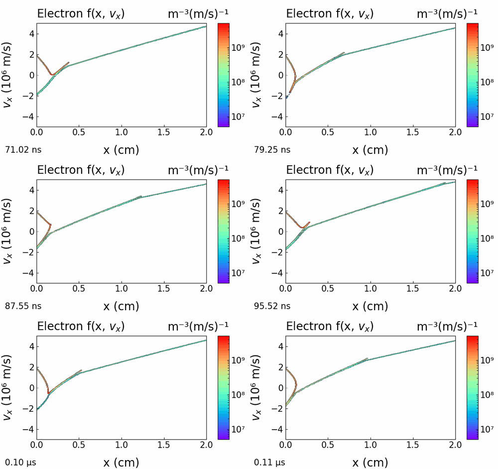
Figure 104: Phase space (x,vₓ) of the electrons

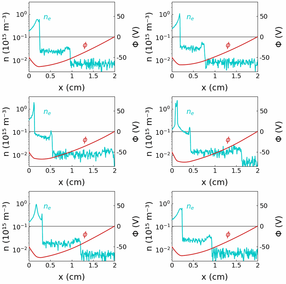
Figure 105: Time evolution of the electron density and electric potential profiles (the two figures are not synchronized).

IV.B Thermionic Discharges

Thermionic discharges are a fundamental class of plasmas. They are driven by the continuous emission of electrons from a heated cathode into a background gas. Unlike an idealised vacuum diode, they are governed by a complex interaction between the injected electron beam, the neutral gas, and the positive ions generated self-consistently. An accurate description of the emission is essential for setting the plasma-sheath boundary. Thermally emitted electrons enter the system with a flux-weighted mean velocity $(\pi/2)^{1/2}\, v_{th}$, where $v_{th}$ is the electron thermal velocity. After injection, they are accelerated, undergo ionising collisions, and build an ion population. This ion population fundamentally changes the space-charge distribution and the potential structure across the discharge gap. The literature on thermionic discharges is extensive. Here we focus on kinetic models of the low-pressure, low-current regimes.

The Emission Current: Richardson-Dushman

The maximum emission current density that a hot cathode can supply is set by its temperature through the Richardson-Dushman law:

where $\phi_W$ is the cathode work function and $A_G$ is the Richardson constant. This emission can be further increased by the Schottky effect or by field emission. In the models presented here we prescribe a fixed temperature for the emitted electrons. For simplicity, the injected current is not coupled self-consistently to the electron temperature or to the local field at the cathode.

Operational Regimes

The steady-state behaviour of a thermionic gas discharge is determined by the applied potential, the gas pressure, and the resulting ionisation rate. This leads to several distinct and well-documented modes [65-66,70-73].

In the Temperature-Limited Mode (TLM), a sufficiently high voltage produces rapid volume ionisation of the gas. The resulting ion space charge neutralises any electron accumulation near the emitter and establishes a classical ion-rich cathode sheath. The current is then limited only by the thermal emission capacity of the cathode, which is set by its temperature, and not by the applied voltage. A related Langmuir Mode (LM) is often seen as an intermediate state with a lower current. It is characterised by a virtual cathode (a local potential minimum) whose negative space charge limits the extracted electron current. This mode is therefore space-charge-limited. In collisional plasmas the LM is inherently unstable: charge-exchange collisions trap ions in the potential minimum, and the increase of the trapped ion density moves the discharge toward the Anode Glow Mode.

When the emitted current exceeds a threshold at low pressure, the TLM with Beam-Plasma Instability develops. It transfers kinetic energy from the directed beam into high-frequency longitudinal Langmuir waves.

At low current the discharge can instead enter the Anode Glow Mode (AGM). Its characteristic feature is the formation of an inverse cathode sheath: cold ions are trapped near the emitter, while the primary ionisation is strongly localised in a thin, highly luminous layer close to the anode.

Finally, the AGM is intrinsically unstable. It shows low-frequency self-oscillations (“self-spikes”), which are observed both experimentally and in PIC-MCC simulations. Greiner et al. proposed that these spikes come from a kinetic instability of the potential distribution, a bounded-plasma Pierce-Buneman instability. However, the precise mechanism is still a subject of active research. An example is described in detail in this section.

IV.B. Case 1 Temperature Limited Mode (TLM)

Discharge Dynamics and Potential Structure

When the applied voltage is high enough, the thermionically emitted electrons are quickly accelerated across the gap. They gain a kinetic energy much larger than the ionization threshold of the gas. This produces volume ionization in the whole bulk. The resulting high density of positive ions determines the potential structure of the discharge.

In the Langmuir Mode (LM) and in the Anode Glow Mode (AGM), a negative space charge exists near the emitter [72]. In the TLM, the dense population of positive ions completely neutralizes this negative space charge [65]. As a result, no virtual cathode forms. Instead, an ion-rich cathode sheath develops. The potential increases monotonically, or with a sharp positive jump, directly from the cathode surface into the bulk plasma. This strong electric field immediately accelerates every emitted electron away from the cathode surface. The whole emitted current is therefore extracted.

Emission Saturation and Total Discharge Current

The main characteristic of this mode is the saturation of the primary electron emission. The positive space charge removes any potential barrier, so the extracted thermionic current is no longer limited by the space charge. Instead, the primary injected current density saturates at the value fixed by the cathode temperature and material. This value is given by the Richardson-Dushman equation. However, in a gas the total discharge current does not remain perfectly constant when the voltage increases, as it would in an ideal vacuum diode. A higher anode voltage gives a higher kinetic energy to the electrons that cross the gap. This increases the rate of volume ionization across the gap. The new electron-ion pairs add to the total measured current. In the standard TLM, the total current remains of the same order of magnitude as the primary emitted current. Because the gas pressure is usually low, the number of ionizing collisions per primary electron is small. This ionization is enough to produce the slow positive ions needed to neutralize the electron space charge at the cathode, but it does not produce a large avalanche. As a result, the total discharge current is only slightly larger than the thermionic emission limit. This clearly separates this regime from fully developed thermionic arcs.

Figure 106: Spatial profiles of electron and ion densities and electric potential at steady state. The conditions of the simulations are given below.

Figure 107: Steady-state electron (x, ε) phase space. Electrons are emitted with a Maxwellian flux at 0.25 eV and are accelerated to 40 eV by the applied potential drop across the cathode sheath. A clear 20 eV energy gap separates the primary beam from the bulk electrons. This gap exists because the lowest inelastic excitation thresholds in helium are approximately 20 eV, so the beam electrons lose exactly this quantity of kinetic energy in a collision. The phase space also shows a small spatial modulation of the beam energy, which indicates Langmuir waves. These wave structures can become much stronger at higher emitted electron currents (see “TLM with Beam-Plasma Instability” in this section).

Conditions of the simulation

Helium at p=2 Pa Gap length d=15 cm Cathode voltage V=-40 V Current density of emitted electrons Jₑ₀=0.2 A/m² Temperature of emitted electrons Tₑ=0.25 eV (the current and the temperature of the emitted electrons are fixed separately, for simplicity) Initial conditions: - Plasma density 10¹⁴ m⁻³ - Number of grid points 400 - Number of particles 100000 - Time step 5x10⁻¹¹ s

IV.B. Case 2 Beam-Plasma Instability in a Thermionic Discharge

This study considers a collisional, self-sustaining thermionic discharge [65]. The applied potential is high enough to keep the system strictly in the temperature-limited mode (TLM). This prevents the formation of a virtual cathode and any transition to the Anode Glow Mode (AGM).

Physical Mechanism

In low-pressure thermionic discharges, electrons are emitted from a heated cathode and then accelerated across the cathode sheath. This injects a strongly directed, almost monoenergetic beam into the bulk plasma. Under some conditions, this can create a strongly non-equilibrium, bump-in-tail Velocity Distribution Function (VDF). As this beam propagates through the colder, quasi-neutral background plasma, it starts a kinetic two-stream (or beam-plasma) instability.

This instability is a collective relaxation mechanism. It transfers kinetic energy from the directed beam into high-frequency longitudinal Langmuir waves. In a bounded, self-sustaining discharge, this wave-driven thermalization is not a simple, steady-state progression in space. It competes with collisional damping, it is strongly modulated by spatial density gradients, and it is coupled with the macroscopic electrostatic potential. This coupling often drives the entire discharge into a strongly non-linear, self-sustaining relaxation cycle [70].

Conditions of the simulation

Helium at pressure p=0.67 Pa (5 mTorr) Gap length d=15 cm Electron emission at cathode Jₑ₀= 2 A/m², Half Maxwellian flux at Tₑ=0.25 eV (the current and the temperature of the emitted electrons are fixed separately, for simplicity) Initial conditions: - Plasma density 10¹⁴ m⁻³ - Number of grid points 512 - Number of particles 200000 - Time step 5x10⁻¹² s

Under these conditions, the discharge operates in a self-sustaining regime. It has a macroscopic background plasma with an approximately sinusoidal density profile, with a maximum of about 2x10¹⁴ m⁻³ in the center of the gap.

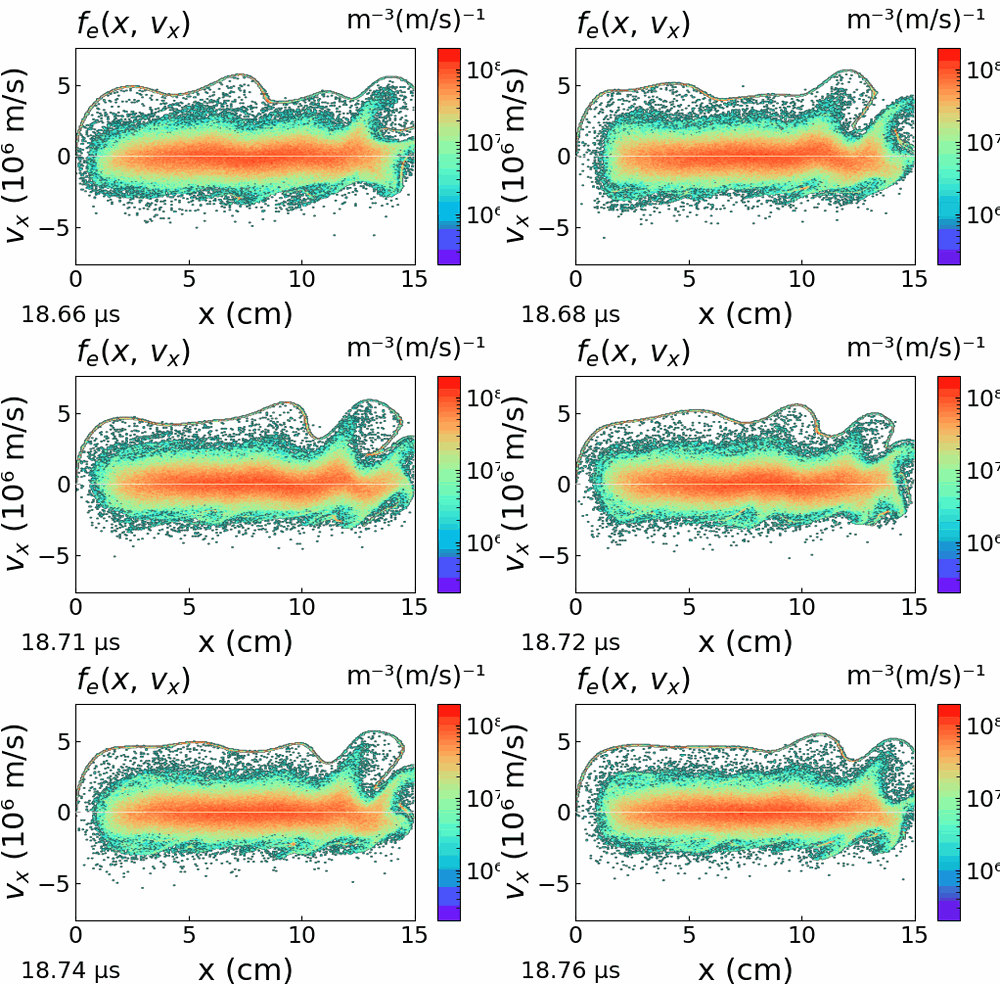
Figure 108: Time evolution of the electron (x,vₓ) phase space showing the beam-plasma instability in the bounded plasma of a thermionic discharge at low pressure. See the kinetic analysis of the instability below.

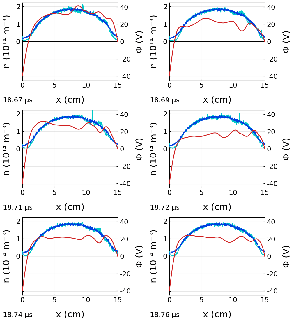
Figure 109: Time evolution of the spatial profiles of the electron and ion densities and electric potential. The large amplitude oscillations of the plasma potential are superimposed on the development of Langmuir waves.

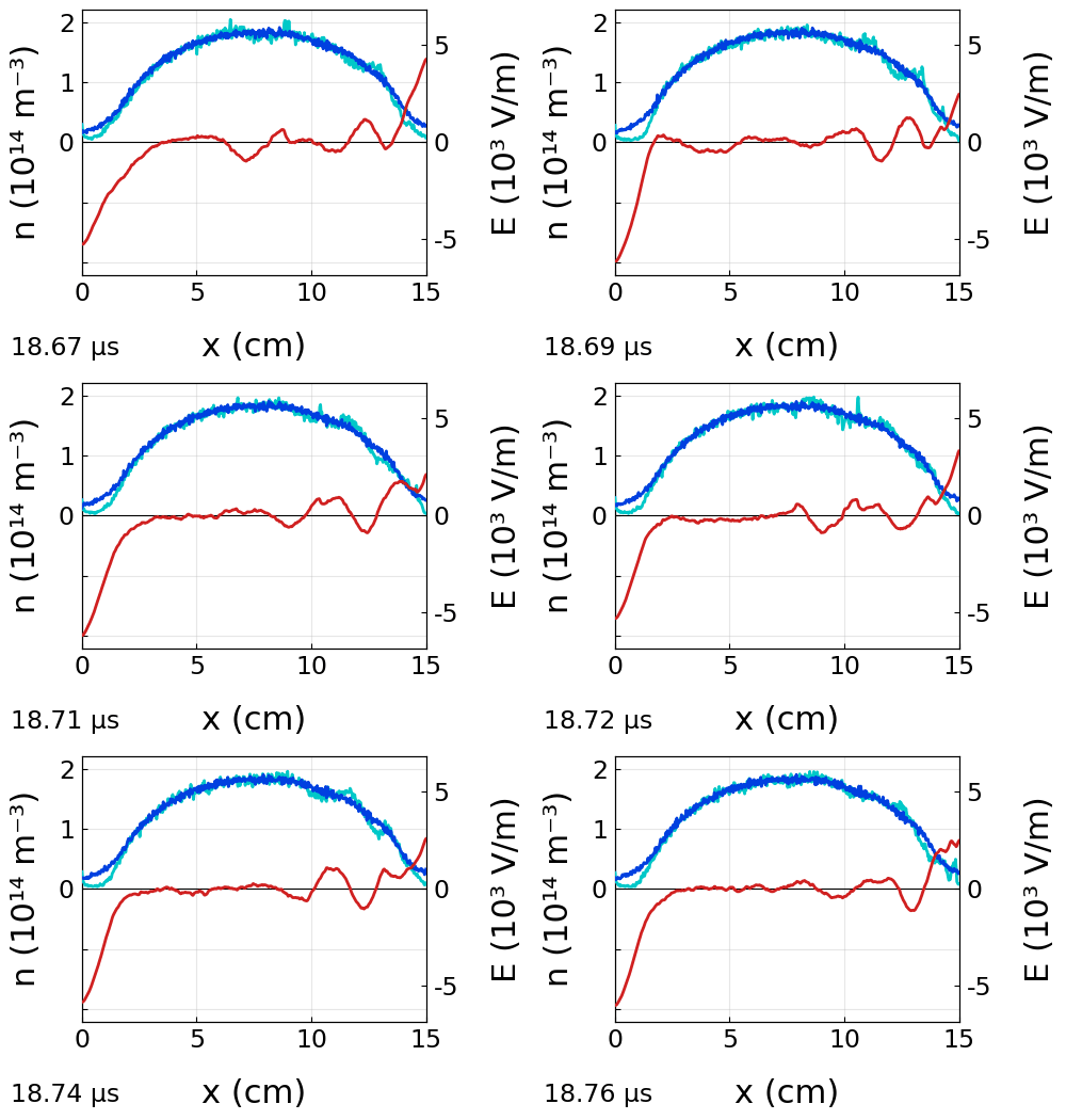
Figure 110: Time evolution of the spatial profiles of the electron and ion densities and electric field.

Characteristic Parameters of the Instability

From the macroscopic parameters, the theoretical properties of the beam-plasma instability can be estimated:

Beam Velocity: Electrons accelerated across the 40 V sheath enter the bulk plasma with a directed kinetic energy of approximately 40 eV. This corresponds to a beam velocity $v_b \simeq 3.75\times10^{6}$ m/s. Oscillation Frequency: The instability couples resonantly with the local electron plasma frequency. At the peak density of 2x10¹⁴ m⁻³, the Langmuir wave angular frequency ωₚₑ is approximately 8x10⁸ s⁻¹. Resonant Wavelength: The wave-particle coupling is strongest when the phase velocity of the wave is equal to the beam velocity. The expected spatial wavelength is therefore $\lambda = 2\pi v_b / \omega_{pe}$, of the order of 2.9 cm. Collisional Competition: At 5 mTorr in helium, the mean free path of 40 eV electrons is about 30 cm, twice the gap. The beam crosses the plasma almost without collisions, so collisional damping is much weaker than the growth of the electrostatic waves. For this reason the instability develops very strongly here. At 15 mTorr and with ten times less emitted current (the previous TLM case), it is only a weak modulation of the beam.

Kinetic Analysis of the Instability

The non-linear nature of the beam relaxation and its coupling to the global discharge dynamics are observed with phase space and field diagnostics. They show three distinct coupled mechanisms: Density Gradients and Delayed Resonance The position where the instability starts is determined by the macroscopic plasma density profile. The instability needs a strict phase coherence between the beam velocity and the local plasma frequency to transfer energy into the Langmuir waves. In the first segment of the discharge, x < 5 cm, the strong positive density gradient continuously changes the local plasma frequency, and this breaks the resonance condition. As a result, the beam remains in a ballistic, laminar state over several centimeters. The resonance condition is maintained long enough only when the beam reaches the density plateau (10 cm< x< 14 cm), where the gradient is zero. There the wave electric field grows exponentially into the non-linear regime. The Anodic Mirror and Cavity Resonance The physical boundaries change the instability from a convective mode to an absolute mode. The plasma potential shows large amplitude oscillations. The reason is that the very mobile electrons tend to escape to the anode faster than the heavier, slower ions. To keep the overall quasi-neutrality, the bulk plasma raises its potential well above the applied voltage, and this creates a repulsive barrier at the anode which confines its own electrons. This high positive bulk potential strongly increases the acceleration of the primary electron beam injected from the cathode. This in turn drives a strong beam-plasma instability and stochastic heating in the plasma volume. The physical mechanism is correct, but the extreme amplitude and the sudden character of these oscillations are artificially amplified by the limitations of the 1D PIC-MCC model. In a real laboratory experiment, radial ambipolar diffusion to the cylindrical chamber walls would continuously remove the excess ions and electrons, and this would damp the increase of the potential. In addition, the perfectly rigid DC voltage boundary condition of the simulation ignores the internal resistance and inductance of a real power supply. Without an external circuit to absorb the transient current peaks, the 1D numerical plasma must sustain an exaggerated collapse of the potential. Anomalous Heating and the Relaxation Cycle The high plasma potential strongly changes the energy balance. The bulk potential reaches +45 V while the cathode remains at -40 V, so the primary electrons in fact fall through an effective potential drop of more than 80 V. When these very energetic electrons enter the non-linear wave region, they are trapped in large phase-space vortices. Stochastic heating in these fluctuating wave fields generates a supra-thermal tail, and a fraction of the electron population reaches energies well above 100 eV. This anomalous heating starts a macroscopic relaxation cycle. The sudden increase of the electron kinetic energy allows a very large flux of electrons to cross the repulsive barrier at the anode. This momentary short-circuit of the space charge produces a fast collapse of the plasma potential, down to +10 V within 50 ns. Once the excess energy has been removed to the anode, the barrier forms again, the ions accumulate again, and the potential increases again. This drives the discharge in a self-sustaining cycle of disruption and relaxation.

IV.B. Case 3 Anode Glow Mode (AGM)

The Anode Glow Mode (AGM) is a separate operating regime of thermionic gas discharges at low current [65]. In this regime the source of electron emission and the main zone of ionization are completely separated in space.

The AGM usually appears from the Langmuir Mode because of collisions [72]. At the beginning, the space charge of the emitted electrons creates a virtual cathode near the emitter, that is a local minimum of the potential [73]. Charge-exchange collisions produce slow and cold positive ions, and these ions are trapped in this potential well. The density of the trapped ions increases slowly. The ions neutralize the local negative space charge and change the potential profile of the discharge.

This change of the potential gives the main feature of the AGM: the formation of an inverse cathode sheath. Near the emitter the potential becomes flat or is reversed. The bulk plasma is then a passive transport region with a low field. In this region the electrons do not gain enough energy to produce ionization in most of the volume.

As a result, the applied electric field is strongly compressed into a narrow region next to the anode, and it forms an inverse anode sheath. The electrons that drift through the bulk are accelerated quickly only when they reach this strong potential gradient. The main ionization by electron impact is therefore located only at the anode boundary. It creates the thin and very luminous plasma layer, the “anode glow”, which gives its name to this operating mode.

This is shown in the figures below. They give the time evolution of the electron and ion phase space (x,vx). They also give the spatial profiles of the electron and ion densities, of the potential, of the mean electron energy and of the ionization rate.

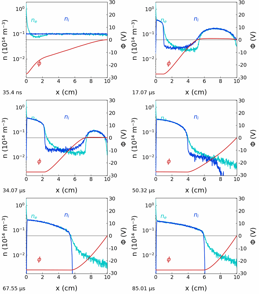
Figure 111: Time evolution of the spatial profiles of the electron and ion densities (log scale) and of the electric potential (the parameters of the simulation are given below). The sequence starts with the formation of a virtual cathode near the emitter. Ions are trapped in this potential well, the local ion density increases and moves toward the anode, and it carries electrons with it to keep quasineutrality. At the end of this evolution, an anode sheath rich in electrons is formed, and the main ionization is confined to a narrow layer next to the anode.

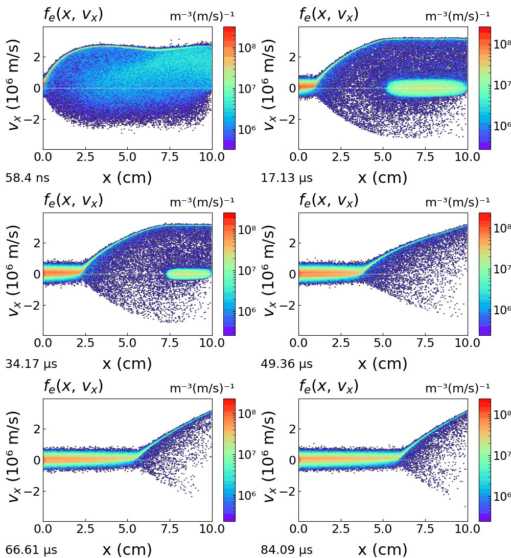
Figure 112: Time evolution of the electron (x, vₓ) phase space. The electron temperature stays low in the quasineutral plasma while it expands. The electrons are accelerated in the region of increasing potential that moves toward the anode, and the ionization takes place there.

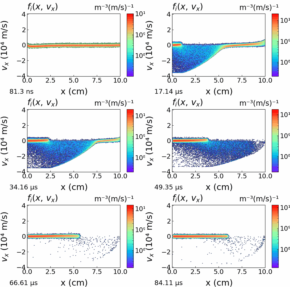
Figure 113: Time evolution of the ion (x, vₓ) phase space. The ions are produced by ionization inside the strong potential gradient that moves toward the anode. They are then accelerated toward the cathode, and they lose kinetic energy by charge-exchange collisions with the background neutral gas.

Figure 114: Time evolution of the mean electron energy and of the ionization rate across the discharge gap. The profiles show that the active ionization region moves away from the cathode region, and that it is finally confined to a thin layer near the anode.

Conditions of the simulation

Helium at pressure p=8 mTorr (1.067 Pa) Gap length d=10 cm Cathode voltage V=-27 V Emitted electron current Jₑ₀=3 A/m² Temperature of the emitted electrons Tₑ=0.25 eV (The emitted current and the temperature are fixed separately, to keep the model simple) Initial conditions - Plasma density 10¹³ m⁻³ - Number of grid points 512 - Number of particles 200000 - Time step 5x10⁻¹¹ s

IV.B. Case 4 Anode Glow Mode (AGM) Self-Oscillations

The Anode Glow Mode (AGM) looks steady, but it often shows periodic low-frequency disturbances. They are called potential relaxation oscillations, or “self-spikes” [66]. Older models often explained these fluctuations by the Pierce-Buneman instability [70-71], but the exact physical cause is still discussed. Campanell and Umansky (2017) also point out that these periodic events are not a change from one macroscopic operating mode to another. They are transient instabilities that develop entirely inside the established AGM.

The origin of this oscillatory behavior is the formation and the evolution of an internal potential double layer (DL). The evolution of this internal DL produces a self-sustaining cycle of disruption and relaxation. Campanell and Umansky [65] describe this cycle as follows:

Double Layer Expansion and Enhanced Ionization: When the internal DL becomes stronger, it gives a large kinetic energy to the thermionic electrons that cross the gap. When the potential difference of the DL becomes larger than the ionization energy of the gas, volume ionization starts in a large region. This changes the usual AGM profile for a short time, because the ionization zone extends far beyond its normal position near the anode.

Ion Feedback and Current Surges: At the same time, the internal electric field of the DL pushes the new positive ions back toward the electron emitter. This return flow of ions increases the ion density at the cathode. It therefore neutralizes the electron space charge that normally limits the emission. As a result, the potential barrier disappears, and a short and strong burst (or “spike”) of thermionic electron current flows through the discharge.

Collisional Damping and System Reset: The collisions between ions and neutrals limit this current burst. A part of the returning ions reaches the cathode surface, but many of these ions make charge-exchange (CX) collisions with the background gas during their motion. These collisions remove the kinetic energy of the moving ions, so the ions are trapped again near the emitter. These slow ions accumulate and rebuild the initial space-charge potential well. The electron burst then stops, and the discharge returns to its normal AGM state until the next instability begins.

The figures below show the self-sustaining cycle of disruption and relaxation obtained in this case. The operating conditions are the same as those of the “Anode Glow Mode (AGM)” case. The only difference is that the present calculation is extended over several hundred microseconds.

Figure 115: Time evolution of the ion density profile during the relaxation oscillations. The conditions of the simulations are given below.

Figure 116: Current as a function of time during the AGM self-oscillations. The figures below show the time evolution of the plasma properties during the disruption and the relaxation, in the time interval 350-400 μs.

Figure 117: Time evolution of the electron and ion densities and of the electric potential, during one cycle of disruption and relaxation between the times 350 and 400 μs

Figure 118: Time evolution of the (x,vₓ) ion phase space during one cycle of oscillation.

Figure 119: Time evolution of the (x,vₓ) electron phase space during one cycle of oscillation.

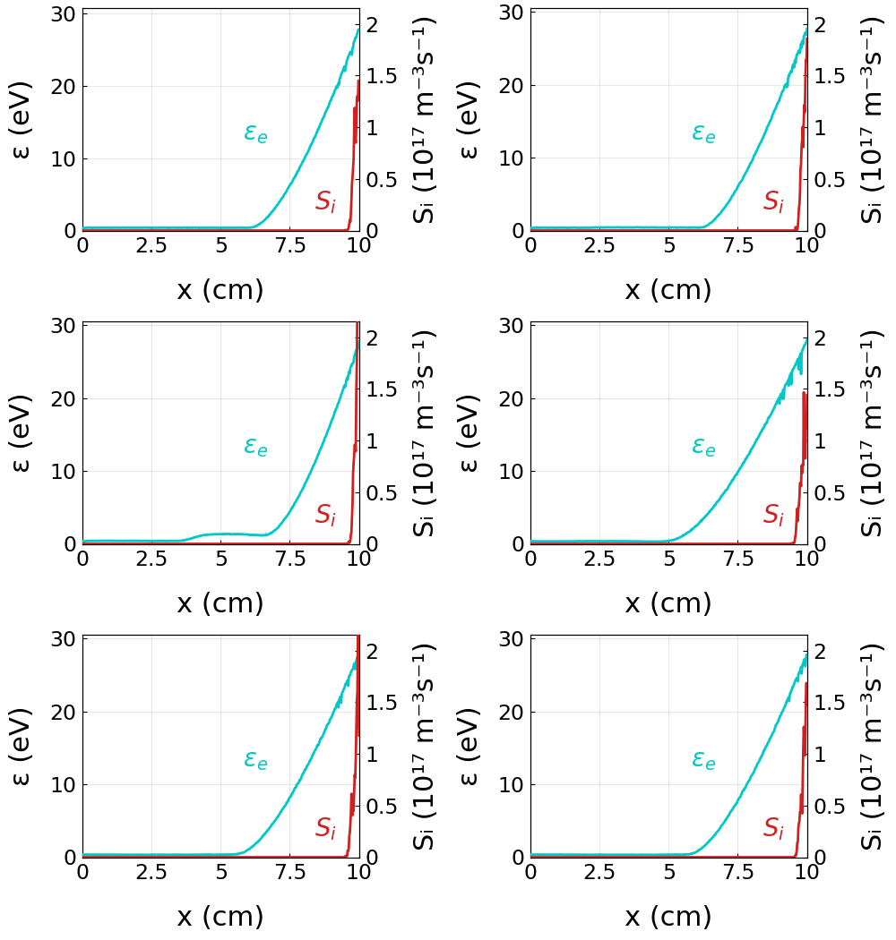
Figure 120: Time evolution of the mean electron energy and of the ionization rate during one cycle of oscillation.

Conditions of the simulations

The conditions of the simulations are the same as those of the “Anode Glow Mode (AGM)” case (extended over several hundred microseconds). Helium at pressure p=8 mTorr (1.067 Pa) Gap length d=10 cm Cathode voltage V=-27 V Emitted electron current Jₑ₀=3 A/m² Temperature of emitted electrons Tₑ=0.25 eV (The emitted current and the temperature are fixed separately, to keep the model simple) Initial conditions Plasma density 10¹³ m⁻³ Number of grid points 512 Number of particles 200000 Time step 5x10⁻¹¹ s

V DC and Transient Glow Discharges

The Direct Current (DC) glow discharge is the basic configuration in which a constant potential difference sustains a steady-state plasma. In a typical glow discharge the pd product (gas pressure times gap length) is of the order of a few Torr·cm. The pressure goes from a fraction of a Torr to several Torr, and the gaps are of the order of a centimetre. Operation at higher pd products, for example at atmospheric pressure with gaps of a centimetre or less, is very useful for industrial applications. It remains a major difficulty, because spatial non-uniformities appear and because there is a risk of transition from glow to arc.

The plasma is sustained self-consistently by ionization in the volume and by secondary electron emission produced by ion impact on the cathode [5,45,74]. In space it is organised in distinct and well-defined regions [75-76]:

• The Cathode Fall — a region of high electric field, where the ions are accelerated towards the cathode and the electrons are accelerated towards the bulk.
• The Negative Glow — a quasineutral bulk controlled by non-local electron kinetics. The high-energy electrons accelerated across the cathode sheath lose their energy here, and they produce strong excitation and ionization.
• The Faraday Dark Space — located immediately after the negative glow. It contains low-energy electrons that do not have the energy needed to excite or ionize the gas, so it is optically dark.
• The Positive Column — a long, uniform and quasineutral plasma. The local electric field adjusts itself exactly to compensate the losses of charged particles to the walls and the electron-ion recombination in the volume.

The positive column is treated in a separate chapter. The present chapter deals with the dynamics of the cathode sheath and of the negative glow.

DC discharges reach a stable equilibrium that does not depend on time, but many practical applications use transient glow discharges. In these discharges a high-voltage pulse is applied quickly. It destroys the initial equilibrium, and the plasma sheath propagates and expands rapidly into the surrounding space. An important example, which combines transient behaviour and the kinetics of high-voltage sheaths, is Plasma Immersion Ion Implantation (PIII). A substrate placed in a background plasma is biased with high-voltage negative pulses. The sudden decrease of the voltage repels the electrons and opens a wide time-dependent ion-matrix sheath. The ions are accelerated across this sheath, they bombard the substrate surface and they are implanted in it.

These discharges contain non-Maxwellian energy distributions, strong gradients of the electric field, and interactions between the particles and the surfaces. A fully kinetic approach is needed to describe them, and the PIC-MCC method is well adapted to this. This chapter presents PIC-MCC examples. They illustrate the changes of structure of DC glow discharges, the expansion of transient sheaths in time, and the controlled ion trajectories that are central for technologies such as PIII.

V.A DC Glow Discharge

This section deals with the cathode fall and the negative glow regions of a glow discharge.

In a Direct Current (DC) glow discharge, the Cathode Sheath (or Cathode Fall) and the Negative Glow are the two most important regions, and they are strongly coupled. Together they maintain the electron multiplication that keeps the plasma alive. The general physics of glow discharges can be found in many textbooks and published papers [5,45,74-76]. This physics has been understood for decades, and the DC glow discharge may look like a relatively simple object. However, its self-consistent kinetic simulation, and that of the negative glow in particular, is difficult, for the reasons given in the Simulations section below.

Physics

This section gives a detailed description of the physics, the structure and the particle dynamics in these two regions.

The Cathode Sheath (Cathode Fall)

The Cathode Sheath is a narrow region located immediately next to the cathode surface. It is characterized by a large drop in potential (the cathode fall voltage) and a strong, non-uniform electric field. Space Charge Dynamics: Because electrons are very mobile, they are quickly removed from this region toward the plasma bulk. This leaves a dense cloud of slow positive ions, which creates a strong positive space charge. Electric Field Profile: This space charge changes the electric field. The field is maximum at the cathode surface and decreases almost linearly to zero at the boundary of the Negative Glow. Particle Mechanics: Ions are strongly accelerated toward the cathode. When they hit the surface, they release secondary electrons by kinetic or potential emission. Secondary Electrons: once in the gas phase, they are accelerated away from the cathode by the high electric field. Because the field is very strong and the distance is short, these electrons are not in local equilibrium with the electric field. Instead, they behave as a high-energy beam.

The Negative Glow

The Negative Glow begins where the strong electric field of the cathode sheath decreases to almost zero. It is the brightest part of the discharge.

Non-Local Electron Kinetics [77]: The high-energy electron beam accelerated across the sheath enters this region with its maximum kinetic energy. Because the electric field here is very weak, these “runaway” electrons are no longer accelerated. Instead, they undergo many inelastic collisions with the background gas.

Ionization and Excitation Cascade: When the beam electrons collide with gas atoms or molecules, they produce a cascade of secondary ionizations and intense electronic excitation. This volume ionization creates a dense, quasineutral plasma bulk. The relaxation of these excited atoms produces the characteristic intense light emission (this is the origin of the name “glow”).

Electron Populations: The Negative Glow usually contains an electron energy distribution function (EEDF) with several components: - Fast beam electrons coming from the sheath. - Electrons that have undergone one or a few inelastic collisions - Ultimate (thermal) electrons that have been cooled by many collisions. These electrons have lost most of their energy, so they are trapped in the shallow potential well formed by the maximum of the plasma potential in the Negative Glow. They can leave the well, and so be lost to the boundaries, only if a collisional mechanism brings some of them back to an energy high enough to pass the confining barrier (see the Simulations section). This trapping produces the very low electron temperature Tₑ and the high plasma density that characterize this region.

The Feedback Loop (Sustainment Mechanism)

These two regions depend strictly on each other: If the cathode sheath does not accelerate the electrons enough, volume ionization in the negative glow decreases. Fewer ions then return to bombard the cathode, secondary electron emission decreases, and the discharge stops. The thickness of the sheath adjusts itself exactly so that each electron leaving the cathode produces just enough ions to release exactly one replacement secondary electron. This condition is called the self-sustained discharge criterion, and it is written:

where M is the electron multiplication in the gap, α is the Townsend coefficient, d is the gap length, and γ is the secondary electron emission coefficient due to ion bombardment of the cathode.

Simulations

The PIC-MCC method is well suited to the simulation of the cathode fall and the negative glow regions of a glow discharge. This is a strongly non-equilibrium kinetic problem, and the electron energy distribution functions (EEDFs) are very different from a Maxwellian. Fluid models rely on closure relations that impose the shape of the EEDF, so they cannot describe the kinetics of this regime.

However, an accurate calculation of the plasma properties in the negative glow, such as the plasma density and the electron temperature, remains a real challenge, even for PIC-MCC simulations [78]. The negative glow is characterized by a high plasma density and a very low temperature of the bulk electron population (measured to be as low as 0.1 eV [79]). In addition, the low-energy electrons are trapped in the local potential well formed by the maximum of the plasma potential in this region. This trapping is central to the problem. A trapped electron can escape, and the negative-glow density can be limited, only if the electron is scattered back to an energy high enough to pass the confining barrier. The dominant de-trapping mechanism is electron-electron (Coulomb) collisions. These collisions diffuse the cold electrons in velocity space and continuously refill the high-energy tail that escapes from the well. An insufficient or missing de-trapping therefore leads directly to an over-estimated density. Because of the very low temperature and the correspondingly long confinement time, the bulk population is extremely sensitive to this set of interactions: electron-electron (Coulomb) collisions above all, but also superelastic collisions and stepwise ionization from metastable states.

As a result, the calculation of an accurate electron energy balance is very difficult, but the resulting plasma density depends strongly on the exact electron temperature. In addition to this physical complexity, there is a major numerical difficulty. The grid-based fluctuations of the electric field and of the potential, which are inherent to the PIC-MCC method, can produce non-physical numerical heating of the cold bulk electrons. If this numerical noise is not controlled, it artificially increases Tₑ and changes the simulated plasma density. A strict spatial and temporal numerical convergence of the simulation method is therefore essential to obtain physically valid results [80-81].

Another major concern is the computation time needed to reach a steady state. The characteristic time scale that governs the plasma density in the negative glow is the ambipolar diffusion time. The ambipolar diffusion coefficient is defined as: $D_a=\mu_iT_e$ As a result, the ambipolar diffusion time scales as: $L_{NG}^2/D_a$ where $L_{NG}$ is the characteristic length of the negative glow. Under the experimental conditions of [79] and with the simulation parameters of [78], Tₑ ≈ 0.1 eV and the helium ion mobility at 3.5 Torr is about 2.5×10³ cm² (V s)⁻¹, so that Dₐ ≈ 3×10² cm² s⁻¹. For a negative glow of length $L_{NG} \simeq 4\ \mathrm{mm}$, the ambipolar diffusion time is about half a millisecond, and the trapped cold population needs several of these times to build up. The convergence time is therefore in the millisecond range [78]. This very long time scale, combined with the difficulty of obtaining an accurate electron energy balance, makes a fully converged, self-consistent particle simulation of the negative glow region very difficult. However, if sufficient care is taken to prevent numerical heating in the glow, particle simulations can still give a reliable estimate of both the electric field profile in the cathode sheath and the total current, even without a fully converged negative glow. Nevertheless, the secondary electron emission coefficient due to ion bombardment is generally poorly known. It must be adjusted to reproduce the experimentally measured current for a given gas pressure, gap length and applied voltage, as done in [78].

Two cases are considered in this section. The first one illustrates the non-local kinetics of the electrons in the cathode sheath and the negative glow [77]. The second one corresponds to a published benchmark simulation of a DC glow discharge [78].

V.A. Case 1 Helium Glow Discharge

Physics

A typical glow discharge is simulated. The gas is helium at 1 Torr and the gap is 4 cm. The cathode region contains the Cathode Sheath and the Negative Glow. It is a useful case for the study of non-local electron kinetics. Helium is a light atom with a high ionization potential (24.58 eV) and high excitation thresholds (19-20 eV).

The simulation conditions of this study are similar to those of Ref. [77]. However, the simulations of Ref. [77] were not self-consistent. They used a pure Monte Carlo method, with an electric field profile across the gap obtained from experiment. This imposed profile is very close to the self-consistent electric field computed by the PIC-MCC simulation of this section.

The thickness of the cathode sheath is only a few electron mean free paths. At high applied voltage it can even be smaller than the mean free path for inelastic collisions. For this reason the electrons emitted by the cathode are accelerated across the sheath to energies much higher than the excitation and ionization thresholds of the gas. In this region the energy gained from the field is much larger than the energy lost in collisions. These fast electrons therefore enter the negative glow as a directed beam. In the “abnormal glow discharge” regime the applied voltage is large and the sheath is thin. The electrons that enter the low-field region of the negative glow then form a well-defined beam, with a peak energy close to the total cathode fall potential. The electrons make very few inelastic collisions in the high-field region, so the cathode sheath remains optically dark.

In contrast, the electric field in the negative glow is very small. The electrons that enter this region no longer gain energy from the field. They lose their kinetic energy quickly, through a dense cascade of inelastic collisions. This strong local excitation produces a very luminous region. The light emission is maximum exactly at the entrance of the negative glow, and it then decreases slowly with the distance from the cathode.

The electrons that have lost all their energy accumulate in the shallow potential well of the negative glow, where they form a cold trapped population. This is the trapping and de-trapping question discussed in the section introduction. At the moderate voltage and pressure used here, this population reaches equilibrium easily and the discharge reaches a well-converged steady state. This case is therefore a clear illustration of the kinetics of the cathode region. The more difficult regime, where a converged negative-glow density is really hard to obtain, is treated in the GD Benchmark case.

The simulation shows the complex structure of the electron energy probability function (EEPF) in typical helium ‘normal glow discharge’ conditions.

Conditions of the simulations

Gas: helium at 1 Torr (300 K) Gap length 4 cm Cathode voltage -160 V Secondary emission coefficient for ion bombardment of the cathode: 0.32 Temperature of the emitted electrons 2 eV Initial conditions: Plasma density 10¹⁴ m⁻³ Number of spatial cells 300 Number of particles 200000 Time step 2×10⁻¹¹ s

Results

Figure 121: Spatial profiles of the charged particle densities (electrons and ions) and of the electric field in the steady state. The transitions between the cathode sheath region and the negative glow region are clearly visible.

Figure 122: Normalized electron energy probability function (EEPF) as a function of position. The complex structure, with several components, shows the strongly non-local electron kinetics of the cathode sheath and of the negative glow.

Figure 123: Normalized EEPF at four different positions in the gap. It shows that several electron populations exist at the same time. In the cathode fall (blue and red curves) a high-energy ballistic group is seen, at the energy given by the local potential. A second group is shifted by about 20 eV, which is the value of the inelastic thresholds of helium. These two groups are the electrons that have made no inelastic collision and the electrons that have made exactly one. Deep in the negative glow (green and orange curves) the progressive relaxation of the electron energy by many inelastic collisions is clearly seen. These results agree with the Monte Carlo simulations of Ref. [77].

V.A. Case 2 GD Benchmark — Carlsson et al.

This case reproduces the DC helium glow-discharge benchmark of Carlsson et al. [78].

Objective of the benchmark

Carlsson’s study had two goals. (i) A code-to-code benchmark between two independent particle-in-cell / Monte-Carlo (PIC-MCC) codes, EDIPIC and LSP, run under exactly the same conditions. (ii) A validation of both codes against a well characterised laboratory experiment. Three applied voltages were simulated, over the whole accessible range: 173 V, 211 V and 600 V. The ion-induced secondary-electron-emission (SEE) yield γ was used as a free parameter. For each voltage it was adjusted to reproduce the cathode current measured in the experiment.

The reference experiment

The reference for the validation is the parallel-plate helium glow discharge of DenHartog, O’Brian and Lawler [79], called the “Lawler experiment”. This experiment is used throughout the benchmark: helium at 3.5 Torr, water-cooled aluminium electrodes 0.62 cm apart, in the (obstructed) glow regime. With laser-optogalvanic and related diagnostics, that experiment gave axial electric-field profiles resolved in space, together with the electron temperature and the density in the negative glow. Such a complete data set is rare. It reports a very low bulk electron temperature (Tₑ ≈ 0.1 eV) and a maximum negative-glow density of ≈ 5×10¹¹ cm⁻³.

Anisotropic scattering — a central ingredient

One special feature of Carlsson’s model is the treatment of anisotropic electron scattering, and this is the main reason why it was implemented in JC-PIC. Carlsson does not assume isotropic collisions. He uses the Okhrimovskyy screened-Coulomb differential cross section [82], in which the scattering is more and more forward-directed when the electron energy increases. The degree of anisotropy is fixed by a single screening parameter, E_aniso, of the order of 100 eV, but its value is not well known. The model is applied to elastic, excitation and ionization collisions, the last ones with a constant screening length. It deflects both the scattered primary electron and the ejected secondary electron. Anisotropy is important here because of the fast electron beam produced in the cathode fall. In this beam, forward scattering changes the distance the electrons travel, and therefore the amount of ionization they produce.

The negative-glow challenge: trapping, de-trapping and convergence

As said in the section introduction, the difficult part of a glow discharge is not the cathode fall but the negative glow. The low-energy electrons produced there are trapped in the shallow potential well formed by the maximum of the plasma potential, at a temperature that the experiment places near 0.1 eV. A trapped electron can leave the well only if a collision brings it back to an energy above the confining barrier, and this is also what limits the density. The main de-trapping process is electron-electron (Coulomb) collisions. Two consequences follow. First, the negative-glow density is very sensitive to the collision physics. Carlsson reports that EDIPIC and LSP differ by a factor ≈ 2.5 for this density, and that both codes give a value below the experimental one. Second, the time needed to build the population of cold electrons is set by the ambipolar diffusion and by the de-trapping. It can reach the millisecond range, so a fully converged and self-consistent simulation is very expensive.

What we did in JC-PIC

To reproduce this benchmark, each key ingredient of Carlsson’s model was implemented in JC-PIC and verified separately: - the Okhrimovskyy anisotropy model: it reproduces Carlsson’s differential cross section (⟨cos χ⟩) to better than 0.2 % from 30 to 500 eV, and the elastic channel is written in a form that conserves the momentum transfer; - the Opal–Peterson–Beaty (OPB) sharing of energy after ionization [83], with the width parameter B = 15.8 eV taken directly from the tabulated EDIPIC cross-section set: it gives the same secondary-electron energy distribution as EDIPIC; - the tabulated helium cross sections (elastic, combined excitation, ionization), with their magnitudes checked against the literature; - electron–electron (Coulomb) collisions (binary Nanbu / Takizuka–Abe operator): they conserve energy and momentum, and they reproduce the Spitzer/NRL relaxation rate in the conditions of the negative glow.

The 211 V case is given as the stored test case in this folder.

Conditions of the 211 V simulation

Gas: helium at 3.5 Torr (300 K) Gap length: 0.62 cm Cathode voltage: −211 V SEE yield (ion bombardment): γ = 0.28 (the value of Carlsson at this voltage) Temperature of the emitted electrons: 2 eV Anisotropic scattering: Okhrimovskyy model on elastic, excitation and ionization Ionization energy sharing: OPB, B = 15.8 eV Electron–electron Coulomb collisions: on Initial conditions: Plasma density: 5×10¹⁶ m⁻³ Number of spatial cells: 1024 Number of particles: ~10⁵ (still increasing slowly toward the steady state) Time step: 2×10⁻¹² s at the start, then adaptive up to 5×10⁻¹² s

Results — 211 V

Figure 124: Charged-particle densities (nₑ, nᵢ) and axial electric field E near the steady state for the 211 V case. The cathode fall (linear field, x ≲ 0.23 cm) and the quasi-neutral negative glow are clearly separated. The field changes sign just after the sheath edge and forms the shallow well that confines the cold electrons.

The agreement with the benchmark is very good. The table below compares the two quantities reported by Carlsson, the field at the cathode surface E₀ and the width of the cathode fall d_c, for JC-PIC, the two reference codes and the experiment:

Table 1: field at the cathode surface and width of the cathode fall at 211 V, for JC-PIC, the two reference codes and the experiment.

JC-PIC reproduces the cathode field of EDIPIC and LSP to within ≈ 2 % and the width of the cathode fall to within ≈ 0.02 cm. Like both reference codes, it gives a field at the cathode about 10 % above the measured one, as reported in [78]. This run is not yet fully converged, because the number of macroparticles is still increasing slowly. However, the structure of the field and the quantities in the cathode region are already stable and in agreement with Carlsson.

The 173 V case

The 173 V case is the lowest voltage of the benchmark and the easiest one. Its cathode fall is the widest and its negative glow the least dense, so it converges most easily. JC-PIC reproduces well the low-voltage part of the benchmark (173 V and 211 V). The 173 V case is not kept as a stored test case.

The 600 V case — an honest account of an unresolved difficulty

Up to now, the case at the highest voltage has not given a converged result in JC-PIC, and this is stated here openly. Carlsson himself describes the 600 V case as only a partial success. It required an increase of γ to 0.33 and a time step divided by two, to 1 ps. It is also the case where the two reference codes differ most (LSP needed γ = 0.36) and where the negative-glow density is the least certain.

Our attempts used the conditions of Carlsson (He 3.5 Torr, 0.62 cm, −600 V, γ = 0.33, dt = 1 ps, anisotropy on, OPB sharing, Coulomb collisions). The runs reached 150 µs. The result is a negative glow that is much too dense, and this dense glow compresses the cathode fall:

Table 2: the 600 V case after 150 µs (not converged), compared with EDIPIC and the experiment.

To find the cause, a systematic verification was made. Every ingredient of the collision physics was found to be correct: - Anisotropy: the angular distribution of JC-PIC agrees with the Okhrimovskyy formula to better than 0.2 % up to 500 eV. A change of E_aniso from 75 to 100 eV changes the multiplication by ≈ 1 %. - Ionization energy sharing: the OPB distribution with B = 15.8 eV is identical to the one of EDIPIC. - Cross sections: the magnitudes for elastic, excitation and ionization collisions are correct. - Coulomb collisions: the electron–electron operator conserves energy and momentum and reproduces the Spitzer relaxation rate. It de-traps the cold electrons as it should. - Cathode-fall multiplication: a Monte-Carlo calculation of the Townsend multiplication in the measured sheath field gives a self-sustaining cathode-fall width of ≈ 0.29 cm, close to the 0.34 cm of Carlsson. The cross sections therefore do not give too much multiplication.

All these checks give the same conclusion. The difference comes not from the collision physics but from the convergence. The negative-glow density is set by the slow accumulation and de-trapping of the cold electrons, which takes about a millisecond, and 150 µs is at least ten times too short. A test with artificially light ions was made to confirm this. Light ions make the ambipolar transport faster, and therefore the convergence faster, without changing the ionization. In this test the negative-glow density decreased to ≈ 2×10¹¹ cm⁻³, the value of EDIPIC, and the cathode fall became wide again, exactly as this explanation predicts.

A fully converged result at 600 V therefore needs either a much longer integration, or an initial negative glow already close to its steady state. This is left for future work, and this section will be updated when such a result is available.

V.B Plasma Immersion Ion Implantation (PIII)

Plasma Immersion Ion Implantation (PIII) is a versatile surface modification technique. A target is immersed in a plasma and high-voltage negative pulses are applied to it. Unlike traditional beamline implantation, PIII treats the entire surface at the same time. It is therefore well suited to 3D objects with complex geometries, without complex manipulation of the target.

The fundamental physics of PIII is the formation and evolution of a dynamic plasma sheath. When the negative pulse is applied, the electrons are rapidly repelled from the target, and a “matrix sheath” of ions is left behind. These ions are then accelerated by the electric field and strike the surface at high velocities. As the process continues, the sheath expands into the plasma to supply more ions. This expansion is governed by the non-steady-state Child-Langmuir law. On impact, the ions penetrate the substrate through ballistic collisions and create atomic cascades. These cascades modify the surface properties of the material, such as hardness, wear resistance or biocompatibility, depending on the implanted species and the acceleration voltage.

In PIII, the dynamics of the sheath expansion determines the energy distribution and the uniformity of the implantation. The transition between subsonic and supersonic regimes depends mainly on the relation between the sheath expansion velocity vₛ and the Bohm velocity $u_B$ ≈ cₛ = √(kTₑ/M) (the ion sound speed).

If one assumes that, after a short transient, the ion matrix sheath evolves into a Child-Langmuir sheath, an analytical expression for the sheath evolution can be written.

where nₛ is the plasma density at the sheath edge, V(t) is the potential across the sheath and s(t) the sheath thickness. This equation states that the instantaneous Child–Langmuir current (left hand side) is equal to the total ion current supplied at the moving sheath edge (right hand side). This total current is the current of ions uncovered by the sheath motion, $e n_s \, ds/dt$, plus the Bohm current $e n_s u_B$ of ions entering the sheath. This equation is based on simplifying assumptions, but it gives a good description of the sheath expansion. It was derived by Chen [84] to describe the decay of a plasma created between negatively biased walls. It was used by Lieberman and coworkers [5,85] in the case of Plasma Immersion Ion Implantation. It can also be applied to the problem of an expanding sheath in the post-arc phase of a vacuum arc [86].

Two possible situations (supersonic and subsonic regimes) can be distinguished, depending on the relative values of the sheath edge velocity and the sound speed. A complete discussion of the supersonic and subsonic regimes, with detailed analytical solutions, can be found in the paper by Murakami and Nishihara [87].

Supersonic Sheath Expansion

When a very high-voltage pulse with a fast rise time is applied, the sheath first expands at a supersonic velocity vₛ > $u_B$ (≡ cₛ, the ion sound speed). Physics: In this regime, the sheath moves faster than the ion acoustic waves can carry information into the bulk plasma. As a result, the ions are essentially “overtaken” by the advancing electric field before they can be pre-accelerated. In these conditions the thin Debye sheath is a kind of discontinuity. It plays a role similar to the transition layer of a shock wave [87]. Implication: The result is a nearly mono-energetic ion flux during the early phase of the pulse, because the ions are reached by the high-potential boundary while they are still almost at rest.

Subsonic Sheath Expansion

As the sheath extends further into the plasma, its expansion velocity decreases, because the available ions are depleted and the volume increases geometrically. Eventually the expansion becomes subsonic, vₛ < cₛ. Physics: In the subsonic regime, a “pre-sheath” has time to form ahead of the actual sheath boundary. This pre-sheath creates a weak electric field that accelerates the ions toward the sheath at the Bohm velocity before they enter the high-field region. A rarefaction wave propagates in the plasma ahead of the sheath front, at the sound speed [87-88]. Implication: This transition gives a more complex energy spectrum and can affect the “matrix” ion density profiles. In most industrial PIII processes the pulse duration is long enough for the sheath to pass from the supersonic regime to a quasi-steady subsonic state. This transition follows the expansion laws derived from the Lieberman or fluid models.

In this section two test cases are considered. They illustrate the supersonic and the subsonic sheath expansion.

V.B. Case 1 Plasma Immersion Ion Implantation

Supersonic regime

This example considers a uniform plasma of density 10¹⁷ m⁻³. A negative voltage pulse is applied to the cathode. The voltage decreases linearly from 0 to -1000 V in 50 ns, and then remains constant at -1000 V. The gas pressure is 1 mTorr and the gas is helium.

The time evolution of a Plasma Immersion Ion Implantation (PIII) pulse can be divided into three physical phases: the initial matrix phase, the supersonic expansion, and the transition to a quasi-steady subsonic state.

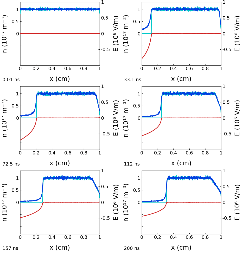
Figure 125: Time evolution of the electron density, the ion density and the electric field during the supersonic phase. The plasma density is 10¹⁷ m⁻³, the applied voltage is 1 kV and its rise time is 50 ns (the detailed conditions of the simulation are given below).

1. The Matrix Phase

The process begins when the negative high-voltage pulse is applied. The electrons have a much smaller mass than the ions, so they are repelled from the target almost immediately. They leave behind a region that contains only immobile ions. This region is called the matrix sheath. At this moment the ions do not move. The electric field only uncovers the ions that are already present in the plasma volume near the surface.

2. Supersonic Expansion (The Voltage Rise)

The potential continues to decrease towards its maximum value, and the sheath expands rapidly into the bulk plasma. In this regime the sheath velocity vₛ is supersonic: it is larger than the ion acoustic (Bohm) velocity cₛ. The sheath moves like a fast piston. It reaches the ions when they are still at rest, before they can react to the electric field that approaches them. These ions are captured and accelerated towards the target with a high energy. Because vₛ > cₛ, no pre-sheath can form in front of the boundary. The plasma is not perturbed until the sheath front arrives. In these conditions the thin Debye sheath is a kind of discontinuity. It plays a role similar to the transition layer of a shock wave.

3. The Plateau and Subsonic Transition

When the voltage reaches its plateau (50 ns in this example), the cause of the rapid expansion disappears. The expansion of the sheath becomes slower, because the sheath must accelerate a mass of ions that increases with time. The velocity vₛ decreases and becomes smaller than cₛ, so the regime becomes subsonic. Ion acoustic waves can then travel in front of the sheath and form a pre-sheath. This pre-sheath accelerates the ions towards the target before they reach the sheath boundary. The system then evolves towards a quasi-steady state described by the Child-Langmuir law. In this state the ion flux is limited by space charge, and no longer by the rapid collection of ions of the supersonic phase.

Figure 126: Contour plots of the time variation of the electron density. The supersonic expansion is visible, and also the transition to the subsonic regime at about 200 ns. Two rarefaction waves then form, one from the cathode and one from the anode, and they merge at about t=700 ns.

Figure 127: Same as Fig. 126, with 1D plots of the electron density profile at different times.

Conditions of the Simulation

Helium at p=1 mTorr (0.133 Pa) Gap length d=1 cm Cathode voltage: linear decrease from 0 to - 1 kV in 50 ns, then constant after 50 ns No secondary electron emission Initial Conditions: Plasma density 10¹⁷ m⁻³ Electron temperature Tₑ=1 eV Ion temperature Ti=0.1 eV Number of grid points 600 Number of particles 2x10⁵ Time step: 2x10⁻¹² s

V.B. Case 2 Plasma Immersion Ion Implantation

Subsonic regime

In this example we consider a uniform plasma of density 10¹⁷ m⁻³. A negative voltage pulse is applied to the cathode. The voltage decreases linearly from 0 to −1000 V in 1 μs, then remains constant at −1000 V. The gas is helium at 1 mTorr. The rise time is 20 times longer than in the supersonic example of this section. So the sheath never enters a strongly supersonic phase, and the expansion remains subsonic during almost the entire pulse.

Physics

Because the voltage increases slowly, the sheath-edge velocity vₛ remains below the ion acoustic (Bohm) velocity $c_s = \sqrt{kT_e/M}$ for most of the pulse. For the present conditions ($T_e$ = 1 eV, helium), $c_s \approx 4.9$ mm/μs. The quasi-static Child-Langmuir sheath only has to grow to $s_C = \frac{\sqrt{2}}{3}\lambda_D (2V_0/kT_e)^{3/4} \approx 3.3$ mm at full voltage ($\lambda_D \approx 23$ μm at 10¹⁷ m⁻³). Reaching this thickness during the 1 μs ramp requires an average expansion velocity of only ~3 mm/μs, which is below $c_s$. The dynamics is therefore an almost quasi-static succession of Child-Langmuir sheaths that follow the instantaneous voltage, $s(t) \approx s_C \left[V(t)/V_0\right]^{3/4}$. It is not the “piston” motion of the supersonic case.

In this subsonic regime the ions have time to respond to the advancing field. A rarefaction wave propagates ahead of the sheath front at the sound speed. A pre-sheath forms, in which the ions are pre-accelerated toward the boundary, and they enter the sheath at the Bohm velocity [87-88]. The sheath motion then follows the non-steady-state Child-Langmuir law introduced at the start of this section [5]. Since $c_s \approx 4.9$ mm/μs, the rarefaction wave launched from the cathode crosses the 1 cm gap in about 2 μs. The grounded anode also draws a Bohm flux through its own (thin) sheath and launches a second, weaker rarefaction wave. The two fronts therefore meet near the middle of the gap at t ≈ 0.85 μs, and the whole plasma density then decays. This is the situation analyzed by Chen [84] for a plasma decaying between negatively biased walls.

As a consequence of the slow ramp, the implanted-ion energy distribution is much broader than in the supersonic case. The ions that cross the sheath during the ramp arrive with all intermediate energies between ~0 and 1 keV. Only the ions collected during the plateau approach the full $eV_0$. The gas is effectively collisionless for the sheath: at 1 mTorr the ion charge-exchange mean free path, ~10 cm, is much larger than the gap. The matrix-ion density profile is correspondingly smoother than in the supersonic regime.

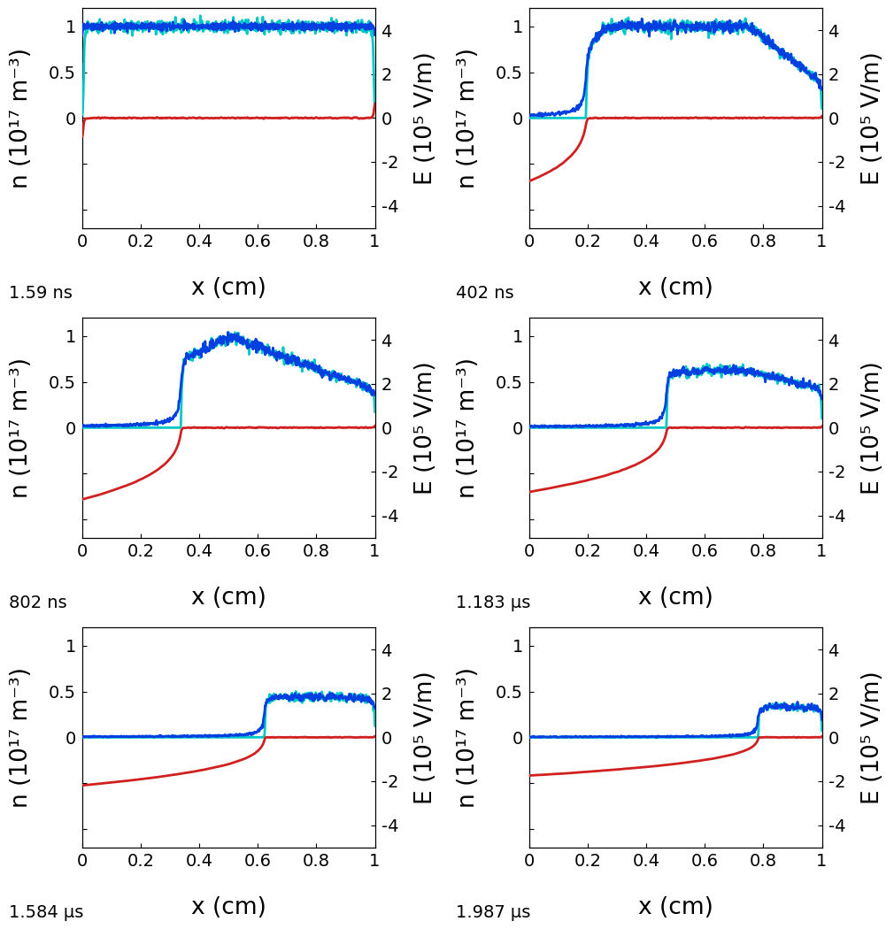
Figure 128: Time evolution of the electron density, ion density and electric field during the pulse (animation). The sheath edge advances smoothly and follows the quasi-static Child-Langmuir thickness of the instantaneous voltage. The density ahead of it is progressively reduced by the rarefaction wave. Compare with the sharp piston-like front of the supersonic case.

Figure 129: Contour plot of the electron density in the position-time plane. The sheath-edge trajectory is a smooth curve whose slope remains below the ion-acoustic slope $c_s \approx 4.9$ mm/μs. The rarefaction fronts launched from the cathode and the anode merge near mid-gap at t ≈ 0.85 μs. After that, the density decays throughout the gap.

Figure 130: Electron density profiles at successive times. Each curve shows the sharp cathode sheath edge advancing into the plasma (the vertical drop to zero on the left), the weak rarefaction gradient on the anode side, and the increasing reduction of the bulk density. The plateau density decreases from 10¹⁷ to about 0.5×10¹⁷ m⁻³ by the end of the pulse. This is the 1D counterpart of Fig. 129.

Figure 131: Ion flux-energy distribution at the cathode (IFEDF), integrated over the whole pulse (t = 2 μs), on a logarithmic vertical scale. Two components appear. The narrow peak near 980 eV collects the ions that fall through the sheath during the −1000 V plateau. They all cross essentially the same cathode fall, so the peak is almost mono-energetic. It is slightly below the full 1 keV because of the pre-sheath and plasma-potential drop, which the ions do not gain. The broad, nearly flat shelf from ~0 to ~950 eV collects the ions arriving during the 1 μs voltage ramp. Since V(t) increases linearly, the instantaneous cathode fall, and therefore the arrival energy, passes uniformly through all intermediate values. This produces an essentially flat energy distribution. This two-part spectrum (a broad ramp shelf plus a plateau line) is the characteristic of the slow, subsonic pulse. It contrasts with the much narrower, nearly mono-energetic distribution of the supersonic case. A logarithmic scale is needed to see the ramp shelf, which is otherwise much smaller than the plateau peak.

Conditions of the Simulation

Helium at p = 1 mTorr (0.133 Pa) Gap length d = 1 cm Cathode voltage: linear decrease from 0 to −1 kV in 1 μs; constant after 1 μs No secondary electron emission Initial conditions: Plasma density 10¹⁷ m⁻³ Electron and ion temperatures 1 eV and 0.1 eV Number of grid points 600 Number of particles 2×10⁵ Time step 5×10⁻¹² s

VI Capacitively Coupled RF Discharges

Capacitively coupled radio-frequency (CCRF) discharges are the main tool of low-temperature plasma processing. In the simplest form a gas at low pressure, from a few mTorr to a few Torr, is confined between two parallel electrodes. One electrode is driven by a radio-frequency voltage, most often at the industrial frequency of 13.56 MHz, and the other one is grounded. The plasma obtained in this way is used in the semiconductor, flat-panel-display and photovoltaic industries for etching, thin-film deposition and surface treatment. It delivers a controlled flux of ions to a surface at a controlled energy.

The RF Regime

The physics of a CCRF discharge is determined by the order of the characteristic frequencies:

The driving frequency is much higher than the ion plasma frequency and much lower than the electron plasma frequency. As a result, the light electrons follow the instantaneous RF field. The heavy ions are too slow to follow it and respond only to the time-averaged field. Sheaths depleted of electrons therefore form in front of each electrode, and their thickness oscillates at the RF frequency. The ions drift steadily towards the electrodes across the time-averaged sheath potential. In the most general case the applied voltage is a tailored waveform with several harmonics,

The classical single-frequency drive (k = 1) is a special case of this waveform. The forms with several frequencies and controlled phases are the basis of several sections of this chapter.

Sheath Dynamics and Electron Heating

The bulk plasma is quasineutral and almost free of electric field. For this reason, almost all the power coupled to the electrons is delivered at the oscillating sheath edges, or just outside them. Three mechanisms exist together. Ohmic (collisional) heating acts wherever electrons drift against a resistive background. Stochastic (collisionless) heating occurs when electrons are reflected by the rapidly expanding sheath and gain energy, as a ball gains energy when it is reflected by a moving wall. This mechanism dominates at low pressure. Finally, moment analyses of the Boltzmann equation show that strong ambipolar fields just outside the sheaths, asymmetric in time, play an important role. Earlier models had underestimated this role. The way the balance between these channels changes with pressure and driving frequency is a central subject of the discharge and of this chapter.

Symmetry, Self-Bias and Independent Control

An old limitation of single-frequency CCRF processing is that the ion flux and the ion bombarding energy are coupled [5]. When the voltage is raised to increase the flux, the energy also increases. The way to separate them is to act on the symmetry of the discharge. If the two sheaths are not equivalent, a DC self-bias appears on the driven electrode. A symmetry parameter compares the maximum voltages that the two sheaths can sustain,

This parameter compares the effective areas of the powered and the grounded electrodes through a model exponent q. The DC self-bias that results is obtained from the extrema of the applied waveform,

Any mechanism that moves ε away from unity therefore produces a self-bias. This self-bias can be adjusted almost independently of the plasma density. Two such mechanisms are studied in this chapter. The first is the Electrical Asymmetry Effect (EAE), in which a tailored two-harmonic voltage breaks the temporal symmetry of the waveform. The second is the Magnetic Asymmetry Effect (MAE), in which an asymmetric static magnetic field parallel to the electrodes breaks the spatial symmetry. Both allow the ion energy to be adjusted at almost constant ion flux.

What This Chapter Illustrates

The sections below reproduce, with JC-PIC, a set of well-documented CCRF studies:

• Benchmarks (Turner et al., 2013) [89] establishes the credibility of the method. Four helium cases were simulated by five independent PIC-MCC codes, and the results agree to better than 0.5%.
• eduPIC (Donkó et al., 2021) [90] studies again reference cases taken from a freely available PIC-MCC code written for teaching.
• Pressure effect (Godyak et al., 1990–1992) [91-92] follows an argon discharge at fixed current over the pressure range where the electron heating changes from stochastic to ohmic. In the same range the EEPF changes from bi-Maxwellian to Druyvesteyn-like.
• Dual frequency (Heil et al., 2008; Donkó et al., 2009) [93-94] shows the EAE and the separate control of ion flux and ion energy by the phase between the harmonics.
• Power absorption (Schulze et al., 2018) [95] analyses the electron heating mechanisms in argon at several pressures, and shows the importance of the ambipolar contribution.
• Frequency effects (Sharma et al., 2018) [96] shows how the driving frequency and the voltage determine the plasma density and the ion energy. It also shows a mode transition above a threshold frequency.
• Magnetized RF (Yang et al., 2017; Oberberg et al., 2018) [97-98] illustrates the MAE, in which a weak asymmetric magnetic field (tens of gauss) produces a self-bias that can be controlled.

Together these cases cover the verification of the method, the basic physics of electron heating, and the two main routes to the independent control of ion flux and ion energy. These two routes are the electrical one and the magnetic one. This independent control is what makes CCRF discharges so useful.

VI.A Benchmark of Turner et al. (2013)

In a 2013 paper, Turner et al. [89] proposed the first benchmark of Particle-in-Cell with Monte Carlo Collisions (PIC-MCC) codes for the conditions of Capacitively Coupled Radio-Frequency (CCRF) discharges. This important paper asked for more rigour in the development and the testing of simulation programs, through clearly described and published verification and validation work. The authors explained that a strong way to build confidence in a simulation is to repeat the calculation with several independent codes and to show that the results agree. For particle-in-cell simulations, this means that the results are statistically indistinguishable.

The benchmark uses four operating conditions of a capacitive RF discharge in helium. All of them have a gap length of 6.7 cm, a driving frequency of 13.56 MHz and a gas temperature of 300 K. In each case the voltage amplitude is chosen to give approximately the same current-density amplitude (~10 A m⁻²). The cases then differ mainly in the gas pressure, which covers a factor of about thirty:

• Case 1 — 30 mTorr (9.64×10²⁰ m⁻³), 450 V
• Case 2 — 100 mTorr (3.21×10²¹ m⁻³), 200 V
• Case 3 — 300 mTorr (9.64×10²¹ m⁻³), 150 V
• Case 4 — 1 Torr (3.21×10²² m⁻³), 120 V

This series has a physical meaning. When the pressure increases, the electron energy relaxation length becomes smaller than the electrode gap. The discharge therefore changes from strongly non-local to local. In case 1 the electron distribution in the bulk remains close to Maxwellian and the ionization is spread over the whole gap. In case 4 the ionization and the power deposition are concentrated in the sheath regions.

For an accurate description of the collisions, the protocol prescribes four electron-neutral cross-sections: elastic momentum transfer, two excitations and one ionization. They are taken from the Biagi 7.1 compilation on www.lxcat.net, with isotropic scattering. The ion-neutral scattering uses the isotropic-plus-backward model of Phelps. The tabulated cross-sections and all the numerical parameters (initial conditions, time steps, particle numbers) are given in the paper and in its electronic supplement.

These four cases were simulated by five separate groups, with PIC-MCC codes developed independently, written in different languages and optimized for different architectures. The results were statistically indistinguishable, and the agreement was better than 0.5% with the prescribed protocol. The cases are therefore a reference for the test of any new code.

The four cases have been reproduced with JC-PIC and are given as ready-to-run test cases in this section. A fifth folder, Case 2 — Current driven, repeats Case 2 with the RF current imposed instead of the voltage, and the code must then return the 200 V. This folder is also the worked example of the current-source drive of JC-PIC. The JC-PIC vs Benchmark folder at the end of the section compares the four runs with the figures of the paper. The main benchmark quantity is the time-averaged ion density profile. JC-PIC reproduces its mid-plane peak to within 0.2% (case 1), 1.6% (cases 2 and 3) and 2.7% (case 4) of the published values. This agreement is excellent, and it validates the collision set, the field solver and the boundary treatment of JC-PIC.

VI.A. Case 1 Case 1 — Helium at 30 mTorr, 450 V

This is the lowest-pressure case of the Turner benchmark, and the one that the benchmark was really designed to test. At 30 mTorr the electron energy relaxation length is longer than the electrode gap. So an electron crosses the whole discharge between two collisions that change its energy appreciably. Its kinetics is therefore non-local: the distribution function at a given point is not determined by the field at that point, and every closure used by a fluid model fails. This is also the case with the lowest plasma density of the four, so a particle code has the smallest statistical margin here. Everything below follows from these two facts.

Simulation conditions

The conditions are those of Ref. [89]. No parameter was adjusted.

• Gas: helium at 9.64×10²⁰ m⁻³ (30 mTorr at 300 K). Four electron-neutral processes from the Biagi 7.1 compilation [99] (elastic momentum transfer, two excitations and ionization) with isotropic scattering. Ion-neutral collisions use the isotropic-plus-backward model of Phelps.
• Geometry and drive: plane-parallel gap of 6.7 cm. A sinusoidal voltage of amplitude $V_{RF}$ = 450 V at 13.56 MHz (period 73.7 ns) is applied to the left electrode; the right electrode is grounded. No secondary electron emission, no external circuit.
• Initial conditions: uniform plasma, electrons at 3 eV, ions at room temperature (0.026 eV).
• Discretisation: 128 cells, 512 particles per cell, time step 1.84×10⁻¹⁰ s.
• Averaging: the profiles below are averaged from 90 µs to the end of the run at 150 µs, that is about 800 RF cycles after the discharge has reached its periodic steady state.

Numerical resolution This must be checked explicitly, because the benchmark has no meaning if the discretisation is not adequate. At the discharge centre $n_e$ ≈ 1.3×10¹⁴ m⁻³, so the Debye length is $\lambda_D$ ≈ 2.0 mm, and the cell size is $\Delta x$ = 0.52 mm: $\lambda_D/\Delta x$ ≈ 3.8. The electron plasma frequency is ≈ 100 MHz, that is $\omega_{pe}/\omega_{RF}$ ≈ 8. The time step resolves the RF period with 401 steps and keeps $\omega_{pe}$·dt ≈ 0.12. Both stability conditions of an explicit electrostatic PIC are satisfied with a margin, and the grid resolves the Debye length instead of only matching it.

Structure of the discharge

Figure 132: Time-averaged profiles of the electron density (cyan), the ion density (blue) and the electric field (red).

The densities have their maximum at the mid-plane, about 1.4×10¹⁴ m⁻³, and they are identical over the central two centimetres: the bulk is quasi-neutral, as required. They separate in the sheaths. At the electrodes $n_i$ is still 3.6×10¹³ m⁻³, a quarter of its central value, while $n_e$ has decreased to 10¹² m⁻³. This factor of thirty-five between the two species at the wall is the time-averaged sheath.

The field profile shows how much of the gap is occupied by this sheath, and the answer is most of it. The field is almost antisymmetric, from −1.6×10⁴ V m⁻¹ at one electrode to +1.6×10⁴ V m⁻¹ at the other. It is below 5 % of its maximum value only between 2.8 and 3.9 cm. The field-free quasi-neutral bulk is therefore only about one centimetre wide out of 6.7, and the time-averaged sheaths occupy more than two centimetres on each side. This geometry is the reason why this case is non-local: an electron accelerated at one sheath edge crosses very little field-free plasma before it meets the other sheath.

Where the electrons are heated, and where the gas is ionized

Figure 133: Time-averaged mean electron energy (cyan, left axis) and ionization rate (red, right axis).

These two curves do not have their maxima at the same place. This is the main point of the case.

The mean energy $\langle\varepsilon\rangle$ has two maxima of 16.2 eV at $x$ = 2.0 and 4.7 cm. These are the mean positions of the sheath edges, where the expanding sheath does work on the electrons. It decreases slightly to 13.8 eV at the centre, and it decreases to 4 eV at the electrodes, where only the slowest electrons of the distribution remain. The small steps visible on this curve inside the sheaths are statistical, not physical: the time-averaged electron density there is two orders of magnitude below the bulk value, so each point is based on far fewer samples.

The ionization rate behaves in the opposite way. Its maximum is at the centre of the gap, 1.0×10²⁰ m⁻³s⁻¹, and its full width at half maximum is 2.4 cm, more than a third of the gap. The electrons are hottest at the sheath edge, but they ionize in the middle. Two effects combine. First, the source term is $n_e S_{iz}$-weighted: the ionization rate is the product of the density, which is maximum at the centre, and a rate coefficient determined by the tail of the distribution. Second, and more fundamentally, the fast electrons produced at the sheath edge do not ionize where they were produced. They cross the bulk first. Figure 134 shows this directly.

Ionization dynamics over one RF cycle

Figure 134: Ionization rate resolved in space and time over one RF period (73.7 ns), averaged over many cycles.

There are two ionization bursts per period, one per sheath expansion, separated by half a cycle: here at about 18 and 55 ns. Their maximum is 1.3×10²⁰ m⁻³s⁻¹. This is the classical signature of sheath-expansion (stochastic) heating [5]. Its period is set by the drive, not by any plasma time scale.

The characteristic feature of the low-pressure case is where the bursts are located. Each maximum is at $x$ ≈ 3.4 cm, in the middle of the gap, far from the sheath that produced it. Followed backwards in time, each burst starts as a weak band that leaves a sheath edge and moves inwards. The group of electrons accelerated by the expanding sheath travels at a few 10⁶ m s⁻¹ and needs a large fraction of the half-cycle to cross the bulk. It ionizes on its way and reaches its maximum ionizing efficiency only well inside the plasma. A local model, which computes the ionization from the field at the same point and the same instant, cannot produce this displacement at all.

The deep blue regions near the electrodes over most of the cycle should also be noted. There the sheath is collapsed, the remaining electrons are cold, and the ionization is not only small but zero.

The electron energy distribution

Figure 135: Electron energy probability function, averaged over the RF cycle and over the gap. A Maxwellian is a straight line on these axes.

Over most of its range this distribution is a straight line. From 5 eV to 60 eV the slope corresponds to a temperature of about 11 eV. This must be compared with the (2/3)$\langle\varepsilon\rangle$ = 9.2 eV obtained from the moments of the profiles. The tail is only slightly hotter than the bulk, and by this measure the electron population is close to Maxwellian.

This deserves a comment, because it is the opposite of what one might expect at the lowest pressure of the series. The decisive detail is the behaviour of the curve at the inelastic thresholds of helium: excitation at 19.8 eV, ionization at 24.6 eV. The curve passes through both of them without a visible break. The population above the excitation threshold is therefore resupplied by the sheaths as fast as the inelastic collisions destroy it. This is exactly what “the energy relaxation length exceeds the gap” means in practice: an electron does not reach equilibrium with a local field. It crosses the whole discharge, and the heating and the losses average out over this path.

The tail extends beyond 60 eV, four decades below the maximum. This small population supplies the ionization of Figure 133. It is also the reason why this case needs many particles: the quantity of most interest is carried by the part of the distribution that is sampled worst. The same plot for the three other cases shows a break at 19.8 eV that becomes a sharper knee as the pressure increases, while the tail shortens from 45 eV at 100 mTorr to below 30 eV at 1 Torr. The comparison is made at the end of each of those descriptions.

Agreement with the benchmark

The time-averaged ion density has its maximum at the discharge centre, $n_i$ ≈ 1.40×10¹⁴ m⁻³. This matches the published benchmark value to within 0.2 %. As expected in the non-local regime, the mean electron energy varies little across the bulk, and the ionization source remains distributed across the gap instead of having maxima at the sheath edges. This is the behaviour expected at the lowest pressure of the series.

The power balance closes independently. The source delivers 125 W m⁻² to the charged particles. The field does 33 W m⁻² of work on the electrons and 90 W m⁻² on the ions; the remaining 2 % is the displacement term. The ions receive nearly three quarters of the power. This is the normal situation in a low-pressure capacitive discharge: the electrons collect the energy, but almost all of it is spent to accelerate the ions across the sheaths, and it is finally deposited on the electrodes.

Summary

Case 1 is the hardest of the four cases for a code to reproduce, and the easiest to understand physically: every figure shows the same thing. The sheaths occupy two thirds of the gap. The electrons are heated at the sheath edges but ionize in the middle. The ionization maximum is delayed with respect to the heating by a fraction of a half-cycle, because the fast electrons must first cross the plasma. And, as the JC-PIC vs Benchmark description shows, the electron power density is negative where the sheath collapses. None of these features survives a local approximation. This is exactly why the benchmark starts here.

The agreement with the published value of the peak ion density, 0.2 % on the primary benchmark quantity, is obtained with the prescribed cross sections, the prescribed discretisation and no adjustment of any kind. The power balance closes independently to 2 %. Together with the three companion cases, whose profiles are compared side by side in the JC-PIC vs Benchmark description at the end of this section, this validates the collision set, the field solver and the wall treatment of JC-PIC over a thirty-fold range of pressure.

The Power absorption section of this chapter goes further in the analysis. It decomposes $P_e$ into its ohmic, pressure-driven and inertial contributions for a related set of conditions.

VI.A. Case 2 Case 2 — Helium at 100 mTorr, 200 V

At 100 mTorr the discharge is three times more collisional than case 1. It is still a low-pressure discharge. The electron energy relaxation length $\lambda_\varepsilon$ is now comparable to the gap $L$ instead of larger than it. This case is therefore in the transition between non-local and local kinetics. For this reason it is the most difficult of the four cases to interpret. Ionization is still maximum at the centre, but the profile has become flatter. The electron distribution is still close to Maxwellian at low energy, but a break has appeared at the first inelastic threshold. The discharge is not yet dominated by the sheaths, and it is no longer the non-local plasma of case 1.

Simulation conditions

The conditions are those of Ref. [89]. No parameter was adjusted.

• Gas: helium at 3.21×10²¹ m⁻³ (100 mTorr at 300 K). Four electron-neutral processes from the Biagi 7.1 compilation [99] (elastic momentum transfer, two excitations and ionization) with isotropic scattering; ion-neutral collisions use the isotropic-plus-backward model of Phelps.
• Geometry and drive: plane-parallel gap of 6.7 cm. A sinusoidal voltage of amplitude 200 V at 13.56 MHz (period 73.7 ns) is applied to the left electrode. The right electrode is grounded. No secondary electron emission, no external circuit.
• Initial conditions: uniform plasma at 5.12×10¹⁴ m⁻³, electrons at 3 eV, ions at room temperature (0.026 eV).
• Discretisation: 256 cells, 256 particles per cell, time step 9.22×10⁻¹¹ s.
• Averaging: the profiles below are averaged over the last 100 µs of a 500 µs run. The discharge reached its periodic steady state long before this window.

Numerical resolution At the centre of the discharge $n_e$ ≈ 8×10¹⁴ m⁻³, so $\lambda_D$ ≈ 0.56 mm against a cell size $\Delta x$ = 0.26 mm: $\lambda_D/\Delta x$ ≈ 2.1. The electron plasma frequency is 257 MHz, that is $\omega_{pe}/\omega_{RF}$ ≈ 19, and the time step gives 800 steps per RF period. Both stability conditions of an explicit electrostatic PIC are satisfied. The grid has been doubled and the time step halved relative to case 1, because the higher density reduces the Debye length and the discretisation must follow.

Structure of the discharge

Figure 136: Time-averaged profiles of the electron density (cyan), the ion density (blue) and the electric field (red).

The plasma has a single maximum and is symmetric. $n_i$ reaches 8.42×10¹⁴ m⁻³ at the mid-plane, six times the density of case 1 for less than half the voltage. Lower voltage and higher density both have the same effect: the sheaths become thinner. The time-averaged field is below 5 % of its peak between 1.4 and 5.3 cm. Each sheath is therefore now about 1.4 cm wide against 2.8 cm in case 1, and the quasi-neutral bulk has grown from 1.1 to 3.9 cm. The electron and ion densities are indistinguishable over this whole bulk and separate only in the last centimetre. At the electrodes $n_i$ is 7.1×10¹³ m⁻³.

This is the first thing to notice about the series. What changes from case to case is not so much the plasma as the fraction of the gap that it occupies.

Where the electrons are heated, and where the gas is ionized

Figure 137: Time-averaged mean electron energy (cyan, left axis) and ionization rate (red, right axis).

The mean energy is remarkably uniform: 6.98 eV across the whole bulk, i.e. $T_e$ = 4.65 eV. There is only a small maximum of 7.11 eV at the sheath edges and a decrease to 1.5 eV at the walls. In case 1, $\langle\varepsilon\rangle$ varied by 20 % between the sheath edge and the centre. Here the bulk is nearly isothermal, because the electrons are collisional enough to share their energy across the plasma.

The ionization rate is still maximum at the centre, but only just. Its value at the centre is 99.4 % of its maximum, and its full width at half maximum is 4.0 cm. The profile has become a plateau covering the entire bulk instead of the pronounced central maximum of case 1. This is the transition itself: the central maximum has not yet split into two peaks at the sheath edges, as in case 3, but it has become almost flat.

Ionization dynamics over one RF cycle

Figure 138: Ionization rate resolved in space and time over one RF period (73.7 ns), averaged over many cycles.

There are two bursts per period, one per sheath expansion, as in case 1. But they have moved. The maxima are now at $x$ ≈ 2.2 cm and 4.6 cm instead of 3.4 cm. Each burst has moved from the middle of the gap toward the sheath that produced it. The electrons heated at the sheath edge still travel a large distance before they ionize, but no longer all the way across the gap.

The bursts are also visibly tilted. Each contour starts near its sheath at about 15 ns and moves toward the centre as time advances, ending near 3.5 cm at about 40 ns. This slope is the propagation of the group of heated electrons. Its inclination measures directly how far the electrons travel before they thermalize. A fluid model cannot represent this quantity.

Between the two bursts the ionization does not decrease to zero anywhere in the bulk, unlike case 1. The plasma is collisional enough that a background of ionization remains over the whole cycle.

The electron energy distribution

Figure 139: Electron energy probability function, averaged over the RF cycle and over the gap. A Maxwellian is a straight line on these axes.

Below 20 eV the curve is straight, with a slope corresponding to 5.0 eV. This agrees with the (2/3)$\langle\varepsilon\rangle$ = 4.65 eV obtained from the moments. Above 20 eV the slope becomes clearly steeper.

This break is not arbitrary: it is at 19.8 eV, the first excitation threshold of helium. Below this energy an electron can only lose energy elastically, a fraction 2mₑ/M ≈ 2.7×10⁻⁴ per collision [5], so it gains energy almost freely by a random walk. Above this energy, one collision costs the whole 19.8 eV. At some point the inelastic mean free path becomes short compared with the distance that an electron travels in a half-cycle. The population above the threshold is then destroyed faster than the sheath can renew it, and the distribution bends.

Case 1 showed no such break: its curve was straight through both inelastic thresholds. Here the break is present but small, and the tail still reaches 45 eV. In cases 3 and 4 it becomes a sharp knee and the tail ends before 35 and 30 eV respectively. The four EEPFs, read in order, are the clearest single diagnostic of the transition that this benchmark was built to cover.

Agreement with the benchmark

The time-averaged ion density has its maximum at 8.42×10¹⁴ m⁻³, within 1.6 % of the published benchmark value of 8.28×10¹⁴ m⁻³. The central electron temperature of 4.7 eV also agrees to a few percent.

The power balance is divided almost equally here. Of the work done by the field on the charged particles, 48 % goes to the ions and 52 % to the electrons. In case 1 the ions received three quarters; in case 4 they will receive one eighth. This case is close to the crossover.

Summary

Case 2 is the least spectacular of the four and, for this reason, the most instructive about the meaning of “transition regime”. Every quantity is half-way. The ionization profile is flat instead of peaked or double-peaked. The mean energy is nearly uniform. The EEPF has a break at the excitation threshold but keeps a long tail. The field does equal work on both species. Nothing has inverted yet, but nothing looks like case 1 any more either.

The side-by-side comparison of the ionization rate and of the two power densities for all four cases, drawn on the axes of Figs. 138, 139 and 5 of Ref. [89], is given in the JC-PIC vs Benchmark description at the end of this section.

VI.A. Case 3 Case 3 — Helium at 300 mTorr, 150 V

At 300 mTorr the discharge has changed regime. The electron energy relaxation length $\lambda_\varepsilon$ is now shorter than the gap $L$, so an electron loses its energy well before it can cross the plasma. The kinetics has become largely local: the discharge is heated and ionized where the field is, not where the density is. The signature is very clear in Figure 141, where the ionization profile has inverted relative to the two lower-pressure cases. The central maximum has split into two peaks located at the sheath edges. In this case the central result of the benchmark becomes visible in a single plot.

Simulation conditions

The conditions are those of Ref. [89]. No parameter was adjusted.

• Gas: helium at 9.64×10²¹ m⁻³ (300 mTorr at 300 K). Four electron-neutral processes from the Biagi 7.1 compilation [99] (elastic momentum transfer, two excitations and ionization) with isotropic scattering; ion-neutral collisions use the isotropic-plus-backward model of Phelps.
• Geometry and drive: plane-parallel gap of 6.7 cm; a sinusoidal voltage of amplitude 150 V at 13.56 MHz (period 73.7 ns) is applied to the left electrode, and the right electrode is grounded. No secondary electron emission, no external circuit.
• Initial conditions: uniform plasma at 5.12×10¹⁴ m⁻³, electrons at 3 eV, ions at room temperature (0.026 eV).
• Discretisation: 512 cells, 128 particles per cell, time step 4.60×10⁻¹¹ s.
• Averaging: the profiles below are averaged over the last 70 µs of a 470 µs run. The discharge has reached its periodic steady state long before.

Numerical resolution At the discharge centre $n_e$ ≈ 1.8×10¹⁵ m⁻³, so $\lambda_D$ ≈ 0.35 mm against a cell size $\Delta x$ = 0.13 mm: $\lambda_D/\Delta x$ ≈ 2.7. The electron plasma frequency is 380 MHz, that is $\omega_{pe}/\omega_{RF}$ ≈ 28, and the time step gives 1600 steps per RF period. The grid is four times finer than in case 1 and the time step four times shorter. This is the cost of a plasma fourteen times denser.

Structure of the discharge

Figure 140: Time-averaged profiles of the electron density (cyan), the ion density (blue) and the electric field (red).

$n_i$ reaches its maximum of 1.84×10¹⁵ m⁻³ at the mid-plane, thirteen times the density of case 1 at one third of the voltage. The profile is no longer the smooth bump of the low-pressure cases. It is a broad dome with clearly flattened shoulders.

The sheaths have become narrower again. The time-averaged field is below 5 % of its peak value between 0.99 and 5.71 cm, so each sheath is about 1 cm wide and the quasi-neutral bulk occupies 4.7 cm. This is seven tenths of the gap, against one sixth in case 1. The field itself is essentially confined to these two layers. Over the whole bulk it cannot be distinguished from zero on this scale. This is exactly the condition under which a local description starts to make sense [5].

Where the electrons are heated, and where the gas is ionized

Figure 141: Time-averaged mean electron energy (cyan, left axis) and ionization rate (red, right axis).

The mean energy is flat at 5.92 eV across the bulk, that is $T_e$ = 3.95 eV. It has small maxima of 6.10 eV at the sheath edges and decreases to 0.8 eV at the electrodes. The bulk is isothermal to better than 3 %.

The ionization rate has inverted. Instead of one central maximum it now has two, of 6.1×10¹⁹ m⁻³s⁻¹ at 1.3 and 5.35 cm, exactly where the mean energy has its maxima. They are separated by a central minimum at 51 % of this value. The sequence is the following: case 1 had a pronounced central bump, case 2 a flat plateau, and here the profile has turned inside out.

The reason is that the two factors in $S_{iz}$ have changed their relative weight. The rate is the product of $n_e$, which still has its maximum at the centre, and a rate coefficient set by the tail of the distribution. This coefficient now has sharp maxima at the sheath edges, because the electrons no longer carry their energy away from the place where they gained it. At 300 mTorr the second factor dominates.

The ionization has not disappeared at the centre: half of the peak value remains, so the bulk still contributes substantially. The inversion is complete but not yet extreme. That is case 4.

Ionization dynamics over one RF cycle

Figure 142: Ionization rate resolved in space and time over one RF period (73.7 ns), averaged over many cycles.

There are two bursts per period, as always, but now they are clearly attached to their sheaths. The maxima are at $x$ ≈ 1.25 cm at 27 ns and 5.5 cm at 62 ns, within a few millimetres of the sheath edges identified in Figure 140. Their peak value, 2.1×10²⁰ m⁻³s⁻¹, is 1.6 times that of case 1, even though the applied voltage is one third of it. The ionization is concentrated in a much smaller volume and a much shorter interval.

The residual non-locality is still visible, and this figure is the best place to see it. Each burst has a tail that extends toward the centre of the gap. The fastest electrons of the heated group still escape from their sheath and ionize on their way, and they reach 3 cm before they disappear. This tail produces the non-zero central minimum in Figure 141. It is exactly the part of the physics that a local model would miss.

Over most of the cycle, and everywhere outside these two lobes, the ionization is essentially zero. This is the deep purple that now covers most of the diagram, where case 1 had a continuous green background.

The electron energy distribution

Figure 143: Electron energy probability function, averaged over the RF cycle and over the gap. A Maxwellian is a straight line on these axes.

The break at 19.8 eV, the first excitation threshold of helium, has become a pronounced knee. Below it the curve is straight with a slope of 4.0 eV, in agreement with the (2/3)$\langle\varepsilon\rangle$ = 3.95 eV obtained from the moments. Above it the distribution decreases roughly twice as steeply and reaches the 10⁻⁵ floor by 34 eV.

Compared with the two lower-pressure cases, the trend is monotonic. Case 1 went straight through the threshold and beyond 60 eV. Case 2 showed a small bend and reached 45 eV. Here the knee is sharp and the tail ends at 34 eV. What is measured is the competition between two rates: the rate at which the sheath supplies new electrons above 19.8 eV, and the rate at which inelastic collisions remove them. Raising the pressure increases the second, and lowering the voltage decreases the first. The benchmark does both at the same time.

The practical consequence is severe, because the ionization threshold of helium is at 24.6 eV, beyond the knee. The whole ionization of this discharge is supplied by the small population in the steepest part of the distribution. This is why the ionization profile is much more sensitive to the pressure than the density profile.

Agreement with the benchmark

The time-averaged ion density reaches a maximum of 1.84×10¹⁵ m⁻³, within 1.6 % of the published benchmark value of 1.81×10¹⁵ m⁻³. The central electron temperature of 3.9 eV agrees to the same accuracy.

The power balance has reversed relative to case 1. Of the field work on the charged particles, 75 % now goes to the electrons and 25 % to the ions; in case 1 the ions received three quarters. The total power delivered has increased slightly, from 125 to 127 W m⁻². This is therefore a real redistribution and not a change of scale.

Summary

Case 3 is the case where the point of the benchmark becomes visible without any analysis: the ionization profile has two peaks instead of one. Everything else follows from the same cause. The bulk is isothermal because the electrons are collisional. The sheaths are reduced to one centimetre. The distribution function has a sharp knee at the excitation threshold. In the power balance the electrons now take three quarters.

What has not happened yet is the complete disappearance of bulk ionization. Half of the peak rate remains at the centre, and the X-T map still shows the electron groups escaping from their sheaths. The last case completes this evolution.

The side-by-side comparison of the ionization rate and of the two power densities for all four cases, on the axes of Figs. 142, 143 and 5 of Ref. [89], is given in the JC-PIC vs Benchmark description at the end of this section.

VI.A. Case 4 Case 4 — Helium at 1 Torr, 120 V

At 1 Torr this is the case of the benchmark with the highest pressure, the most collisions and the largest computational cost. It closes the series at the opposite end from case 1. The electron energy relaxation length $\lambda_\varepsilon$ is now much smaller than the gap $L$. An electron heated at a sheath edge loses its energy within a few millimetres, so the kinetics is fully local. The ionization is concentrated in two narrow layers next to the electrodes. To a very good approximation, it is absent from the four central centimetres of the discharge. Case 1 and case 4 use the same gas, the same gap and the same frequency, but they behave like two different devices.

Simulation conditions

The conditions are those of Ref. [89]. No parameter was adjusted.

• Gas: helium at 3.21×10²² m⁻³ (1 Torr at 300 K). Four electron-neutral processes from the Biagi 7.1 compilation [99] are included: elastic momentum transfer, two excitations and ionization, with isotropic scattering. Ion-neutral collisions use the isotropic-plus-backward model of Phelps.
• Geometry and drive: plane-parallel gap of 6.7 cm. A sinusoidal voltage of amplitude 120 V at 13.56 MHz (period 73.7 ns) is applied to the left electrode; the right electrode is grounded. No secondary electron emission, no external circuit.
• Initial conditions: uniform plasma at 3.84×10¹⁴ m⁻³, electrons at 3 eV, ions at room temperature (0.026 eV).
• Discretisation: 512 cells, 64 particles per cell, time step 2.30×10⁻¹¹ s.
• Averaging: the profiles below are averaged over the last 250 µs of a 1250 µs run. At that time the discharge has reached its periodic steady state long before.

Numerical resolution At the discharge centre $n_e$ ≈ 2.5×10¹⁵ m⁻³, so $\lambda_D$ ≈ 0.28 mm against a cell size $\Delta x$ = 0.13 mm: $\lambda_D/\Delta x$ ≈ 2.2. The electron plasma frequency is 452 MHz, that is $\omega_{pe}/\omega_{RF}$ ≈ 33, and the time step gives 3200 steps per RF period. The run needs 1.25 ms of simulated time, eight times more than case 1. The reason is that the discharge converges on the ion transit time, and the ions are slower and more collisional here than in any other case of the series. This is 5×10⁷ time steps, and it is the reason why this case is the expensive one.

Structure of the discharge

Figure 144: Time-averaged profiles of the electron density (cyan), the ion density (blue) and the electric field (red).

$n_i$ reaches 2.64×10¹⁵ m⁻³, the highest density of the series. More important than the value, the profile is no longer a dome but a plateau. It is flat to within a few percent over the central four centimetres, and then it decreases abruptly. This shape is the signature of a plasma whose ionization source is at its edges and not at its centre.

The sheaths are the thinnest of the four cases. The time-averaged field is below 5 % of its peak between 0.69 and 6.01 cm. Each sheath is therefore 7 mm wide, and the quasi-neutral bulk occupies 5.3 cm, four fifths of the gap. Across the series the sheath width has decreased from 2.8 cm to 0.7 cm, while the plasma density has increased by a factor of nineteen. These two facts are the same statement, because the sheath thickness scales with the Debye length and with the applied voltage, and both have decreased [5].

At the electrodes $n_i$ is still 1.9×10¹⁴ m⁻³, comparable to the central density of case 1.

Where the electrons are heated, and where the gas is ionized

Figure 145: Time-averaged mean electron energy (cyan, left axis) and ionization rate (red, right axis).

The mean energy is 5.46 eV at the centre, i.e. $T_e$ = 3.64 eV, the coldest bulk of the series. It increases to 6.03 eV in two sharp maxima at 0.52 cm from each electrode, and it decreases to 0.7 eV at the walls. The variation across the bulk is only about 10 %. The two maxima are now narrow peaks instead of the broad maxima of case 1.

The ionization rate is entirely confined to the sheath edges. There are two peaks of 1.42×10²⁰ m⁻³s⁻¹ at 0.75 and 5.95 cm. At the centre of the gap the rate is 0.8 % of that value: it is not “reduced”, it is effectively zero. Case 3 still had half of its peak rate at the centre; here there is nothing.

This is the local limit. The electrons ionize exactly where they are heated, because they cannot carry the energy anywhere else. The plasma that fills the middle of the gap is not produced there at all. It is produced in two thin layers at the edges and diffuses inward. The flat density plateau of Figure 144 is the direct consequence.

Ionization dynamics over one RF cycle

Figure 146: Ionization rate resolved in space and time over one RF period (73.7 ns), averaged over many cycles.

When this map is compared with the same figure for case 1, the whole benchmark is summarised in one image. In that figure there are two broad diamonds that cover the middle of the gap and half of the cycle. Here there are two compact spots at $x$ = 0.75 cm at 27 ns and 6.0 cm at 64 ns, and nothing at all anywhere else. The ionization is localised in space, to less than one centimetre, and in time, to about a fifth of the period.

The peak rate, 7×10²⁰ m⁻³s⁻¹, is five times that of case 1. The same discharge current has to be sustained through a volume an order of magnitude smaller, and during a shorter fraction of the cycle.

A weak plume still extends from each spot toward the centre, up to perhaps 2 cm. This is the last remnant of non-local transport. Even at 1 Torr it has not disappeared completely: a small fraction of the heated electrons still escapes from its sheath. A local fluid model would set this fraction to zero. Whether this matters depends on what is computed. It does not have a measurable effect on the density here, but it is the population that produces the fast-electron tail seen in Figure 147.

The electron energy distribution

Figure 147: Electron energy probability function, averaged over the RF cycle and over the gap. A Maxwellian is a straight line on these axes.

The knee at 19.8 eV, the first excitation threshold of helium, is at its sharpest, and the tail beyond it disappears. The distribution reaches the 10⁻⁵ floor at 27 eV, whereas case 1 was still above 10⁻⁴ at 60 eV. Below the threshold the curve is straight with a slope of about 3.9 eV, close to the (2/3)$\langle\varepsilon\rangle$ = 3.64 eV given by the moments.

The four descriptions of this section now contain the same plot for the same gas at four pressures. Read in order, they make the clearest single statement of the benchmark. Case 1: straight through both inelastic thresholds, tail beyond 60 eV. Case 2: a small bend at 19.8 eV, tail to 45 eV. Case 3: a sharp knee, tail to 34 eV. Case 4: knee and cut-off, tail gone by 27 eV.

The physical content is a competition between two rates: the sheath supplies electrons above the threshold, and inelastic collisions remove them. The benchmark increases the pressure by a factor of thirty, which accelerates the removal. It lowers the voltage from 450 to 120 V, which slows down the supply. Both act in the same direction. The distribution function records their combined effect more directly than any moment of it can.

The consequence for the ionization is the following. The threshold is at 24.6 eV, beyond the knee. In this case the entire ionization of the discharge is therefore produced by a population three decades below the peak of the distribution, in its steepest part. This is why a Maxwellian assumption, which would be acceptable for the density and the temperature here, would be very wrong for the source term.

Agreement with the benchmark

The time-averaged ion density peaks at 2.64×10¹⁵ m⁻³, within 2.7 % of the published benchmark value of 2.57×10¹⁵ m⁻³. This is the largest deviation of the four cases, and it is the expected one, because this run has the fewest particles per cell (64) and the longest integration. The central electron temperature of 3.7 eV agrees to a few percent.

The power balance has completed its reversal. Of the field work on the charged particles, 88 % goes to the electrons and only 12 % to the ions, against 27 % / 73 % in case 1. The total power delivered has more than doubled, from 125 to 284 W m⁻².

Summary

Case 4 is the local limit of the series and the clearest illustration of what that means. The ionization is confined to two layers seven millimetres wide and a fifth of a cycle long. The density profile is a flat plateau, produced entirely at the edges and filled by diffusion. The bulk is isothermal at 3.6 eV. The tail of the electron distribution is cut at the first excitation threshold. In the power balance the ions have become almost negligible.

Compared with case 1, with the same helium, the same 6.7 cm gap and the same 13.56 MHz, this case also shows the value of the benchmark itself. Two operating points of one device differ only in pressure and voltage. They produce discharges with opposite ionization profiles, opposite power balances, and distribution functions that have no common feature except their low-energy slope. A code that reproduces both, with no adjustment between them and with the same cross sections, has demonstrated something that a single well-chosen test case never could.

The side-by-side comparison of the ionization rate and of the two power densities for all four cases, on the axes of Figs. 146, 147 and 5 of Ref. [89], is given in the JC-PIC vs Benchmark description at the end of this section.

VI.A. Case 5 Benchmark of Turner et al. (2013)

Case 2 driven by the current — imposing J(t), reading V(t)

In the four cases of the Turner benchmark the voltage across the discharge is imposed, and the current is part of the result. This case reverses Case 2. The gas, the pressure, the gap, the frequency and the numerical resolution are the same, but the RF current density is imposed and the voltage becomes an output of the simulation. There is a physical reason to use the benchmark in this way. Turner et al. [89] chose the voltage amplitudes of the four cases so that all of them carry nearly the same current-density amplitude, about 10 A m⁻². Driving the series at fixed current is therefore a natural form of the benchmark.

This case has two purposes. It is a worked example of the current source drive of JC-PIC. It is also a closure test with a known answer: the current measured on Case 2 at 200 V is imposed, and the code must return the same 200 V.

Conditions of the Simulation

• Capacitive RF discharge in helium, identical to Case 2: gas density 3.21×10²¹ m⁻³ (≈0.1 Torr at Tg = 300 K), gap length L = 6.7 cm, frequency 13.56 MHz, no secondary electron emission
• Same numerical resolution: 256 grid points, 256 particles per cell, time step 9.0×10⁻¹¹ s, end time 320 µs, initial plasma density 10¹⁴ m⁻³
• Drive: current source — J(t) = J₁ cos(2πf t), with J₁ = 9.26 A/m². This is the fundamental measured on the fully converged voltage-driven Case 2 (see “Building the case” below)
• A change between voltage source and current source requires a Fresh Start

How the current source works in JC-PIC

JC-PIC uses an ideal RF current source, following the method of Verboncoeur et al. [100]. The powered electrode carries a surface charge density σ. The imposed current is given to this electrode in the same way as a real generator would give it. At every time step the analytic integral of J(t) over the step is added to σ. The charge of every particle collected by that electrode, or emitted from it, is added as well. The boundary condition of the field solver at the powered electrode is then not a prescribed potential. It is the Neumann condition E = σ/ε₀. The Poisson solver then gives the electrode potential, that is the voltage, as a result.

This construction has an important property. In a 1D discharge the total current density, conduction plus displacement, is the same at every position, and imposing σ̇ at the electrode imposes exactly that total current. The imposed waveform is therefore satisfied to machine precision at every time step. There is no feedback loop, no regulator and no parameter to adjust. Everything a real current-driven discharge does appears without any extra work. The voltage waveform develops harmonics because the sheaths are nonlinear, and in an asymmetric configuration a DC self-bias builds up in σ, with no iteration on a blocking capacitor. Here the discharge is symmetric, so the bias remains zero. The surface charge is saved in the checkpoint, so a current-driven run can be stopped and continued without a discontinuity.

In the interface the drive is selected on Conditions → Voltage / Current with the Source radio buttons. The three amplitude fields change their names from VDC/VRF1/VRF2 to JDC/JRF1/JRF2 (in A/m²), and the frequencies and the phase are the same as in the voltage mode. In the Currents viewer the curve recorded as the “applied voltage” is now the measured electrode potential. The result of this test case is read there.

Building the case — measuring the current

The imposed amplitude comes from the benchmark itself. Run the voltage-driven Case 2 to its periodic steady state, open the Currents viewer and its FFT window, and read the amplitude of the current fundamental at 13.56 MHz. Only the fundamental is needed. The phase does not matter, because in the steady state it only shifts the time origin, and the harmonics of J are left out on purpose (see below). Then select the current source, enter the measured value as JRF1 and restart from the beginning. The current amplitudes can also be changed while a run is in progress (hot reload), but the type of source cannot. One precaution is required: the measurement must be made on the converged run. As the density increases the sheaths become thinner and carry more displacement current, so the amplitude keeps increasing until the steady state is reached. The converged Case 2 of this library gives J₁ = 9.26 A/m², the value used here. Case 1, which by design should carry the same current, gives 9.78 A/m². The rule of Turner, “same current for all cases”, is therefore exact only to within a few per cent. A first attempt at 9.8 A/m², that is a drive 6% too strong, gave a plasma 6% denser and a voltage 7% higher. This shows how directly the discharge follows its drive.

What to look for

The ignition transient. At the start the initial plasma is much too thin to carry the imposed current by conduction, and a gap with an imposed current behaves as a capacitor. The source increases the voltage toward the vacuum-capacitor limit J₁L/(ωε₀) ≈ 820 V. This continues until the larger field ionizes enough gas for the discharge to carry the current. A current source therefore ignites its own discharge. The voltage then decreases to its steady-state value. The History and Currents viewers show the whole sequence.

The recovered voltage. This is the closure test, and the test succeeds. Driven at the measured 9.26 A/m², the discharge gives a voltage fundamental of 196 V, against the 200 V imposed in Case 2. The difference is 2%, which is the level at which the statistics and the convergence of the two runs can be distinguished. Figure 148 shows the two periods side by side, and the exchange of roles is easy to see. On the left the smooth sinusoid is the imposed voltage, and the clearly flattened curve is the current drawn by the discharge. On the right the smooth sinusoid is the imposed current, and the voltage is the result.

This flattening is the harmonic content of the signal, and it is not the same when the two roles are exchanged. In the voltage-driven case the current has a third harmonic equal to 5.8% of its fundamental. In the current-driven case the voltage obtained has only 1.7%. The nonlinear sheaths distort a current response more than a voltage response. This is a real property of the discharge and not a numerical artefact, and it is the only true difference between the two drives. In both cases the even harmonics and the DC component remain zero, as required by the symmetry of the configuration.

Figure 148: Voltage and total current over one RF period. Left — the voltage-driven Case 2: V(t) is the imposed 200 V sinusoid, and the current is the result, clearly flattened by its third harmonic. Right — this case: J(t) = 9.26 cos(2πft) A/m² is imposed, and the voltage is the result, with V₁ = 196 V and almost no harmonics.

The plasma itself. Figure 149 gives the result that matters. The time-averaged electron and ion densities and the plasma potential of the two runs superpose over the whole gap. Solid lines are the current-driven case, and filled symbols are the voltage-driven Case 2. The peak densities differ by less than 2 % (8.24 against 8.43×10¹⁴ m⁻³). The potential plateau is the same, 100 V, and the sheath widths and the densities at the walls are also the same. Nothing in the plasma depends on which of the two quantities was imposed. This is the physical content of the exercise. A voltage source and a current source are two descriptions of the same generator, related by the impedance of the discharge. The current source of JC-PIC reproduces the benchmark obtained with the voltage source. This is also a useful test of the surface-charge boundary condition itself. A wrong factor in the calculation of σ would appear here as a shift of the density, and no shift is observed.

Figure 149: Time-averaged electron and ion densities (left axis) and plasma potential (right axis). Lines — this case, driven at 9.26 A/m². Filled symbols — the voltage-driven Case 2 at 200 V. The two runs cannot be distinguished.

VI.A. Case 6 JC-PIC vs Benchmark — the four cases side by side

This folder contains no case to run. It gathers the direct comparisons between the four cases of the Turner benchmark and the published results of Ref. [89]. Each of these four cases can be loaded and run from its own folder in this section. The four time-averaged profiles are drawn on one set of axes. This is the most direct way to read the central result of the paper. The figures below use the same quantities and the same axes as Figs. 152, 153 and 5 of Ref. [89], so they can be compared with it directly. The curves are labelled 1 to 4 in order of increasing pressure. The conditions are 30 mTorr / 450 V, 100 mTorr / 200 V, 300 mTorr / 150 V and 1 Torr / 120 V.

Figure 150: Time-averaged ionization rate for the four benchmark cases, to be compared with Fig. 3 of Ref. [89].

This figure defines the series. At 30 mTorr (curve 1) the ionization has a single broad maximum at the centre, 1.0×10²⁰ m⁻³s⁻¹. At 100 mTorr (curve 2) this maximum has become a flat plateau of 0.68×10²⁰ m⁻³s⁻¹ over the central half of the gap. At 300 mTorr (curve 3) the profile is inverted: there are two maxima of 0.61×10²⁰ m⁻³s⁻¹ at 1.3 and 5.4 cm, with a central minimum half as large. At 1 Torr (curve 4) there are two narrow peaks of 1.42×10²⁰ m⁻³s⁻¹ pressed against the sheaths, at 0.7 and 6.0 cm. There is almost no ionization over the middle four centimetres.

This progression, from one central maximum to two peaks at the sheath edges, is the transition from non-local to local kinetics. When the pressure increases, the energy relaxation length $\lambda_\varepsilon$ becomes smaller than the gap. An electron heated at the sheath edge then loses its energy before it can cross the bulk, so it ionizes where it was heated.

Figure 151: Time-averaged power density coupled to the electrons for the four cases, to be compared with Fig. 4 of Ref. [89].

The peak of $P_e$ increases monotonically with pressure. It is about 1.4, 2.2, 3.9 and 7.6 ×10³ W m⁻³ from case 1 to case 4. Its position moves at the same time from 2.25 cm, deep inside the plasma, to 0.5 cm, against the electrode. This is the same result as in Figure 150, shown with the power instead of its consequence.

Two features must be pointed out. In case 1 the electron power is negative near both electrodes, about −1×10³ W m⁻³. In the time average the electrons return energy to the field there. The cause is the collapsing sheath, which decelerates the electrons that its expansion had accelerated half a cycle earlier. This is a purely kinetic effect. A local model, in which the power absorption is proportional to the square of the field, cannot give a negative value anywhere. In case 4 the two sheath peaks stand on a bulk plateau at 2.1×10³ W m⁻³. At 1 Torr the bulk has become collisional enough to sustain ohmic heating across the whole gap, in addition to the sheath heating.

Figure 152: Time-averaged power density coupled to the ions for the four cases, to be compared with Fig. 5 of Ref. [89].

The four curves reach almost the same value at the electrode, 3.3 to 4.0×10³ W m⁻³. This is expected and not surprising. The voltage of each case was chosen so that all four cases run at about the same current-density amplitude. The power density at the wall is close to the product of the ion flux and the sheath field.

What changes with pressure is the width. At 30 mTorr $P_i$ extends over the whole half-gap and reaches zero only at the centre. The sheath is almost collisionless, so an ion is accelerated continuously across it. At 1 Torr the same power is confined to a layer half a centimetre thick against the electrode. The reason is charge exchange, which stops the ions repeatedly, so the ion energy distribution at the wall becomes poorer. The peak value changes very little while the width decreases by one order of magnitude. Therefore the integral, which is the power actually delivered to the ions, decreases strongly with pressure. For case 1 it is 90 W m⁻², three quarters of the total (see the power balance in the Case 1 description).

The two power profiles were integrated for each of the four runs, and this makes the trend clear. The fraction of the field work that goes to the ions decreases monotonically through the series: 73 %, 48 %, 25 % and 12 % from case 1 to case 4. At the same time the total power delivered increases from 125 to 284 W m⁻². Over a change of pressure by a factor of about thirty, the discharge stops being an ion accelerator and becomes an electron heater. This single number describes the whole series better than any of the profiles taken alone. It also explains why the same helium gap at the same frequency behaves as two different devices at the two ends of the pressure range.

A direct comparison of the time-averaged spatial distributions of the electron density between JC-PIC and the benchmark [89] is shown in Figure 153. The agreement is excellent for the first three cases. For the fourth case the JC-PIC values are about 2.7 % below the benchmark.

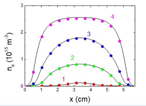
Figure 153: Comparison of the time-averaged spatial distributions of the electron density between JC-PIC (symbols) and the benchmark (solid black lines).

VI.B eduPIC — Donkó et al. (2021)

eduPIC is a compact, spatially one-dimensional electrostatic PIC/MCC code released by Donkó et al. as an educational tool [90]. The paper gives a tutorial on the physical basis and the algorithms of the PIC/MCC technique and makes the full source (in C, C++ and Rust) freely available. Its reference discharge is a single-frequency capacitively coupled plasma in argon: p = 10 Pa, gap L = 25 mm, Tg = 350 K, V₀ = 250 V, f = 13.56 MHz.

The cases in this section reproduce that reference discharge with JC-PIC. Above all, they use it to illustrate one of the most important practical questions of particle simulation: numerical convergence. As shown here, the plasma density and the electron temperature can depend very strongly on the number of grid points and the number of particles per cell.

Why this discharge is so sensitive

The strong sensitivity has a clear physical origin: the Ramsauer minimum in the electron-argon cross-section. Low-energy electrons created by ionization in the discharge centre have a very small collision frequency. Here ν is a few 10⁶ s⁻¹, well below the angular driving frequency ω = 2πf, so that ν² ≪ ω². As discussed by Godyak and Piejak [91], such electrons cannot cross the DC ambipolar potential barrier in the plasma bulk. They need a very long time to reach the oscillating sheath edges where stochastic heating takes place. They therefore remain trapped and cold. This produces the characteristic two-temperature electron energy distribution measured in argon RF discharges.

When the number of particles per cell is too small, fluctuations of the self-consistent field introduce an artificial “numerical scattering”, and numerical heating, which untrap these low-energy electrons. The result is a plasma density that is too low and an electron temperature that is too high. When the resolution is improved (more particles per cell and, because the Debye length becomes smaller, more grid points), the numerical heating is suppressed. The density increases, by almost a factor of two compared with the under-resolved case, and the electron temperature decreases. For these conditions the dependence on the particle number becomes weak above roughly 1000 ions per cell. This also requires 800 grid points instead of 400 to resolve the Debye length. The role of Monte Carlo collisions and of the particle number in this numerical velocity-space diffusion is analysed in detail by Turner [80]. He also notes that electron-electron Coulomb collisions (included neither here nor in eduPIC) would untrap the low-energy electrons in the same way.

What the cases illustrate

The two cases have identical physical conditions and differ only in numerical resolution. Together they show the time-averaged profiles of density, electric field and potential, the electron temperature, the two-temperature EEPF in the plasma centre, and the ion flux-energy distribution (IFEDF) at the electrodes. At the same resolution (400 grid points, ~275 ions per cell) JC-PIC reproduces the eduPIC reference results; the refined case shows the true, converged plasma. The discharge current and the integrated ion flux to the electrodes are only weakly affected by the particle number. The density, the temperature and the low-energy part of the EEPF are strongly affected.

VI.B. Case 1 eduPIC — Donkó et al. (2021)

Reference resolution (400 grid points, ≈275 ions per cell)

This case reproduces the reference discharge of the eduPIC paper [90]: argon at 10 Pa, a 2.5 cm gap, 250 V at 13.56 MHz. It uses exactly the numerical resolution of that paper: 400 grid points and about 275 ions per cell. The case has two purposes. The first is a direct code-to-code comparison at the same resolution. The second is the real subject of this section: the case is the starting point of a convergence study. In this apparently simple argon discharge, the result depends strongly on the number of particles used in the simulation. The Sensitivity/Accuracy case of this section studies this dependence.

The figures below describe the discharge as obtained in this reference-resolution run. The convergence problem is discussed at the end, after the physics.

Conditions of the Simulation

• Capacitive RF discharge in argon, one driven and one grounded electrode
• Gas pressure 10 Pa (≈75 mTorr) at $T_g$ = 350 K, i.e. a gas density of 2.07×10²¹ m⁻³
• Gap length $L$ = 2.5 cm
• Voltage amplitude $V_0$ = 250 V, frequency 13.56 MHz (RF period 73.7 ns)
• No secondary electron emission at either electrode ($\gamma$ = 0), and no electron reflection
• Initial plasma density 1×10¹⁴ m⁻³, initial electron temperature 5 eV

Numerical resolution

• 400 grid points, cell size $\Delta x$ = 62.5 µm
• ≈275 ions per cell, i.e. ≈1.1×10⁵ superparticles per species (superparticle weight 8.0×10⁸)
• Time step $\Delta t$ = 1.84×10⁻¹¹ s, i.e. 4008 steps per RF period
• Run to 350 µs; time averages accumulated after 200 µs, when the discharge has reached its periodic steady state
• The two stability ratios: at the density maximum the Debye length is $\lambda_D$ ≈ 92 µm, so $\Delta x / \lambda_D$ ≈ 0.68, and $\omega_{pe} \Delta t$ ≈ 0.09. Both values are well within the stability limits. For this reason, the convergence problem discussed below is not a resolution problem in the usual sense.

Structure of the discharge

Figure 154: Time-averaged electron and ion density profiles and time-averaged electric field across the gap.

The time-averaged profiles are the classical ones. They are symmetric, as required for two identical electrodes. A quasi-neutral bulk occupies the middle of the gap: between x ≈ 0.44 and x ≈ 2.06 cm the electron density is more than half the ion density. The ion density has its maximum at mid-gap, $n_i$ ≈ 7.2×10¹⁵ m⁻³, and decreases to 3.1×10¹⁴ m⁻³ at the walls. On each side, a sheath about 5 mm thick, almost empty of electrons, carries the whole time-averaged field. This field increases from zero to ±3.4×10⁴ V/m at the electrodes.

The increase is accurately linear, and this deserves a remark. A linear average field means a uniform average space charge. Here it is 2.9×10¹⁴ elementary charges per m³, constant to within a few per cent from the wall to x ≈ 0.6 cm. The time-averaged sheath is therefore very close to a matrix sheath, although the instantaneous sheath is very different (Figure 157).

Inside the bulk the average field is below 1 V/m, four orders of magnitude smaller than in the sheaths. This near-zero field is the reason why the next figure must be examined closely.

Figure 155: Time-averaged electrostatic potential, with the density profiles for reference.

The bulk is at a plateau of 112 V above both electrodes, close to half the applied amplitude. The plateau is flat to a fraction of a volt over one centimetre. But “flat” must be judged against the electron energy scale, not against 250 V. Measured from the discharge centre, the time-averaged potential decreases by 0.3 V at x = 0.8 cm and by 1.7 V at x = 0.6 cm, which is where the electron heating is maximum (see Figure 158). It decreases by 12.4 V at the sheath edge itself. The mean electron energy at the centre is 1.65 eV.

These two numbers, taken together, contain the whole physics of this case. A slow electron created by ionization in the middle of the gap must climb a potential barrier of the order of its own mean energy before it reaches the region where the RF field can heat it. Most of these electrons cannot, and they accumulate. This is the DC ambipolar trapping described by Godyak and Piejak [91]. It produces the cold, over-populated low-energy electron group that is characteristic of argon RF discharges. In argon the trap is unusually effective because of the Ramsauer minimum: these slow electrons have a collision frequency of order 10⁶ s⁻¹, far below the angular driving frequency $\omega$ = 8.5×10⁷ s⁻¹. So collisions neither heat them nor move them across the barrier.

Electron dynamics over one RF period

Figure 156: Electron density over one RF period, logarithmic colour scale.

The two sheaths oscillate in antiphase at the driving frequency. The left sheath collapses completely around t ≈ 0 and t ≈ 70 ns. At these times the electrons reach the electrode itself; this is how the electron current that balances the steady ion current is delivered. At the same times the right sheath is at its maximum width. Half a period later the roles are exchanged. The instantaneous sheath edge travels between the wall and about 0.6 cm in about a quarter of a period, so its velocity is a few 10⁵ m s⁻¹. This is small compared with the thermal velocity of a bulk electron, ≈10⁶ m s⁻¹, but it is not negligible. This is the condition for the moving sheath to transfer energy efficiently to the electrons it reflects.

Figure 157: Electric field over one RF period. The contour lines follow the instantaneous sheath edges.

The field is confined to the sheaths at all times. It is essentially zero in the bulk during the whole cycle: at 10 Pa the bulk conduction current is carried with a negligible field. This is the classical low-pressure, sheath-dominated capacitive discharge. As a result, all the electron heating must take place in the two narrow regions swept by the moving sheath edges.

Where the electrons are heated

Figure 158: Power density transferred from the field to the electrons over one RF period. Red is heating, blue is cooling.

This is the signature of stochastic (sheath expansion) heating, and the map separates its two parts clearly. During the first half-period the left sheath expands and does positive work on every electron it reflects. The whole region it sweeps is red, most intensely close to the electrode, where the expansion starts and is fastest. At the same time the right sheath collapses and gives energy back to the field, along the narrow blue band that follows the retreating sheath edge to the wall. At t ≈ 37 ns the polarity reverses and the two electrodes exchange roles.

The instantaneous values are large, ±6×10⁴ W m⁻³, and the two signs almost cancel. The time average is 4.8×10³ W m⁻³ at the sheath edges and only −14 W m⁻³ at the centre, that is 36 W m⁻² integrated across the gap. There is no visible ohmic heating in the bulk. All the energy received by the electrons is received within a few millimetres of the two sheath edges. This is exactly the region that the trapped low-energy electrons of Figure 155 cannot reach.

Figure 159: Mean electron energy over one RF period.

The result is a discharge with two electron populations, separated in space and in energy. The mean energy reaches 6 eV in the region swept by the expanding sheath. In the time average it is still 3.4 eV at the two sheath edges, and it decreases to 1.65 eV in the bulk, where it almost does not change during the RF cycle. The cold electrons of the centre are not modulated at 13.56 MHz, because nothing reaches them. (The speckled border of the sheaths is not physical. There the electron density is so low that the mean energy is computed from very few superparticles.)

Ionization over the RF cycle

Figure 160: Ionization rate over one RF period; the white lines are contours of the plotted quantity.

Ionization occurs in two bursts per period, one per electrode. Each burst follows the expansion of its own sheath. These are the same events as the red regions of Figure 158, delayed by the time the heated electrons need to travel and to make an ionizing collision. The instantaneous maximum approaches 10²¹ m⁻³s⁻¹. It is reached about a quarter of a period after the sheath begins to expand, some 4 mm in front of the sheath edge and not at the edge itself. This offset is the visible measure of the non-local character of the electron kinetics here: the electrons are heated in one place and ionize in another.

Averaged over the period, this structure largely disappears. The time-averaged ionization rate is 3.1×10²⁰ m⁻³s⁻¹ at the centre and 3.4×10²⁰ m⁻³s⁻¹ at its maximum near x = 1.76 cm. The source is therefore broad and almost flat over the whole bulk. Its integral is 4.7×10¹⁸ ion–electron pairs per square metre per second. A fluid model based on a local mean electron energy would place the source where the energy is, that is at the sheath edges, and would give a wrong profile.

The electron energy distribution

Figure 161: Electron energy probability function, averaged in time, at the middle of the gap.

Everything said so far about trapping is contained in this single curve. The curve has three distinct parts.

Below about 4 eV the distribution decreases very steeply, with an effective temperature of a few tenths of an eV. This is the trapped bulk group: electrons created by ionization in the plasma centre, which cannot climb the ambipolar barrier, and which cannot lose their small energy to argon atoms near the Ramsauer minimum. They simply accumulate. This group contains the large majority of the electrons, and it determines the mean energy of 1.65 eV.

Between about 4 and 12 eV the curve is almost flat: a shoulder rather than a slope. These are electrons that were reflected by an expanding sheath, received a few eV, and have not yet lost this energy. At these energies argon is well above its Ramsauer minimum but still below any inelastic threshold, so only transport removes electrons from this energy range. The shoulder ends near 12 eV, at the first excitation threshold of argon (11.55 eV), as expected.

Above this threshold the distribution again decreases exponentially, with an effective temperature of a few eV, and extends to 50 eV, far beyond the ionization threshold at 15.76 eV. This tail contains about 10⁻⁴ of the population, but it produces all the ionization that sustains the discharge. The energy that dominates the mean is below 2 eV; the energy that dominates the source is above 16 eV. This distance between the two is exactly what makes this discharge so sensitive: a numerical artefact that moves a small fraction of electrons from the first group to the second changes the plasma density substantially, while it is almost invisible in any single-number diagnostic.

Ion bombardment of the electrodes

Figure 162: Ion flux-energy distribution at the electrode.

The ions arrive with a broad spectrum. It has four resolved maxima, at about 7, 25, 48 and 68 eV, on a continuum that ends near 120 eV. This sheath is collisional, not collisionless: the charge-exchange mean free path of Ar⁺ in argon at 10 Pa is about 1.2 mm, and the time-averaged sheath thickness is 5 mm. So a typical ion undergoes several symmetric charge-exchange collisions on its way to the wall. Each collision replaces a fast ion by a slow one at the local potential. The peaks are the groups of ions that made their last collision one, two, three… mean free paths from the wall.

Two numbers complete the picture. The high-energy edge is at the time-averaged sheath drop of 112 V, far below the applied amplitude of 250 V. This is expected: an Ar⁺ ion needs about six RF periods to cross the sheath, so it responds only to the average field. The mean energy delivered per ion, obtained from the wall power and the ion flux, is 34 eV. This is about one third of the 112 V available; the rest is left in the gas by charge exchange.

Power balance

The run also gives the partition of the power drawn from the generator. Integrated across the gap, the field does 36 W m⁻² of work on the electrons and 83 W m⁻² on the ions, so 70 % of the coupled power goes to the ions. Almost all of this ion power is deposited inside the sheaths, where the time-averaged ion power density reaches 1.3×10⁴ W m⁻³ at the electrodes. The budget closes for both species. Of the electron share, 34 W m⁻² is spent in collisions (excitation and ionization) and 4 W m⁻² is carried to the walls by the electrons that escape during the sheath collapse. Of the ion share, 56 W m⁻² goes into charge exchange and elastic collisions in the sheaths, and 26 W m⁻² arrives at the electrodes as ion bombardment. This last quantity is the important one for a sputtering or etching application.

The 70/30 split is characteristic of a low-pressure, strongly capacitive discharge with thick sheaths. It is also the reason why the ion flux-energy distribution at the electrodes is dominated by charge-exchange collisions: an ion crossing the sheath loses about two thirds of the energy it gains before it arrives.

Agreement with eduPIC — and the convergence caveat

With the eduPIC settings, the agreement is excellent. With the same number of cells (400), the same number of particles per cell (≈275) and the same convergence time as Donkó et al., JC-PIC reproduces their reference discharge in every respect: the peak plasma density of 7.2×10¹⁵ m⁻³ against the published $n_\mathrm{max}$ ≈ 7.55×10¹⁵ m⁻³, the central mean electron energy, the sheath thickness and the 112 V potential plateau, the three-part shape of the EEPF, and the multi-peak ion energy distribution at the electrodes. Two independent codes, written separately with different algorithmic choices, give the same discharge.

But these settings are a physical choice here, not a formality. If the convergence parameters are changed (the number of particles per cell, and with it the number of cells), the result changes appreciably. This is the main point of the section, and it is illustrated in the Sensitivity/Accuracy case. With 800 grid points and ≈1000 ions per cell, that is the same discharge with a better resolution, the peak density reaches 1.36×10¹⁶ m⁻³, almost twice the value found here, and the central mean energy decreases from 1.65 to 0.75 eV.

The mechanism is the one analysed by Turner [80]. With ≈275 ions per cell the self-consistent field contains a fluctuating component of purely numerical origin. These fluctuations act on the electrons as an additional, spurious scattering. The population that is damaged is exactly the one that Figures 155 and 161 identified as marginally trapped. If a 1.5 eV electron in the discharge centre receives random kicks of a fraction of an eV often enough, it will eventually climb the 1.7 V barrier, reach the sheath edge and be heated by the real mechanism. Numerical noise empties the trap that the physics fills. As a result the density is too low and the mean energy too high.

None of this appears in the usual stability diagnostics: $\Delta x / \lambda_D$ ≈ 0.68 and $\omega_{pe} \Delta t$ ≈ 0.09 are both fully acceptable here. Reproducing a published reference case at the same resolution is a validation of the code. By itself, it is not a determination of the plasma.

Summary

The reference case is a well-behaved, symmetric, sheath-heated capacitive discharge. Its time-averaged structure, phase-resolved dynamics, electron energy distribution and ion bombardment spectrum are reproduced by JC-PIC in agreement with eduPIC at the same settings. Its interest is that the quantity most users would quote from it, the plasma density, is the one that is not converged. The chain of cause and effect should be remembered, because it appears whenever a discharge has a trapped low-energy electron group. A low collision frequency (here due to the Ramsauer minimum) combined with a small ambipolar barrier produces a population that is sensitive to any spurious diffusion in velocity space. In a PIC code the cheapest source of spurious diffusion is simply too few particles. The remedy is not a finer grid or a smaller time step; it is more particles per cell.

VI.B. Case 2 eduPIC — Donkó et al. (2021)

Sensitivity / Accuracy — the same discharge, well resolved

This case is physically identical to Argon 10 Pa 250 V 13.56 MHz: same gas, same pressure, same gap, same voltage and same frequency. Only the numerical resolution is changed: 800 grid points instead of 400, and about 1000 ions per cell instead of 275. No physical parameter has been modified. Every difference in the result therefore comes from the numerics and not from the plasma. The differences are not small. The steady-state plasma density is almost twice as large as in the case at the reference resolution.

A warning before this case is started: the computation time can become very long. The run holds about 8×10⁵ superparticles per species, about eight times more than the reference case, at the same time step. The discharge still needs about 300 µs to reach its periodic steady state and to average it. This is more than 4000 RF periods, at 4008 steps per period. Depending on the machine, the run takes a large part of a day rather than one or two hours. The checkpoint mechanism allows the run to be stopped and resumed.

How a number of particles per cell is imposed

A PIC-MCC discharge simulation does not run with a fixed number of macro-particles. The run starts with an initial density and an initial number of macro-particles. After that the population evolves on its own. Under the applied RF voltage the discharge ignites, ionization becomes larger than the losses to the walls, and the number of macro-particles increases. The increase is often a factor of ten or a hundred. It depends on how far below the final self-sustained density the initial density was placed. Without a control, the run would fill the particle arrays completely and become very slow long before a steady state is reached. The number of particles per cell, which is the quantity studied in this case, would then be the value the discharge reached by itself. The population must therefore be limited.

The mechanism is called thinning. Two entries of the Initial tab of the Conditions dialog control it. Max # particles is a ceiling on the number of macro-particles. Thinning removal (%) is a depth. At every time step the engine compares the number of macro-particles of each species with the ceiling. When the more numerous species crosses the ceiling, the requested percentage of the macro-particles is removed. In an electropositive discharge this species is the ions. The macro-particles are removed either by a random draw or by a regular stride through the particle array. The storage order has no relation to position or velocity, so the stride gives an equally unbiased sample. Both species are thinned together. The macro-particle weight is immediately rescaled by the exact fraction that is kept. The physical density, the current and the energy content of the plasma therefore do not change during the operation. Only the statistical resolution changes: fewer macro-particles now describe the same plasma.

This is the complete method, and it answers the practical question of this study. A number of particles per cell is imposed by setting Max # particles to that number multiplied by the number of cells. In the run shown below, 800 cells and a target of 440 ions per cell give a ceiling of 352 000. The ≈1000 ions per cell of the present case correspond, on the same grid, to 8×10⁵. Two points must be kept in mind about a number obtained in this way. First, it is a gap average. The plasma is far from uniform, so the cells at the density peak hold clearly more macro-particles than the quoted value, and the sheath cells hold far fewer. Second, it is an upper bound approached from below. Between two thinnings the count covers the band from the ceiling reduced by the removal fraction up to the ceiling itself. With a 10 % removal the mean count is therefore about 5 % below the target, and it never falls more than 10 % below it. The ceiling fixes the particle number only to within the thinning depth. For this reason the depth must be kept small.

Figure 163: Numbers of macro-particles of the two species during a run of the 800-point series, with a ceiling of 352 000 macro-particles (440 ions per cell) and a thinning removal of 10 %. Each vertical fall is one thinning event.

The figure shows the mechanism in operation. The discharge starts with about 5×10⁴ macro-particles per species and ignites in a few microseconds. The count reaches the ceiling almost immediately. The first thinnings then follow one another so closely that they form a solid band. As the plasma approaches its self-sustained density, the growth becomes slower and the events become less frequent. The sawtooth can be read from about 20 µs, and its teeth become steadily wider. The last event occurs at ≈64 µs. After that the count is free. It increases slowly up to about 3.4×10⁵, that is ≈425 ions per cell, and stays there until the end of the run. The small remaining difference between the ion count and the electron count is the positive space charge of the two sheaths.

Each thinning does perturb the run. The plasma is given a coarser description of itself. The statistical noise increases by a factor 1/√0.9 ≈ 1.05, and a few RF periods are needed to return to a steady state. The perturbation is a resampling and not a physical change. No bias is introduced, and the rescaling of the weight conserves the density exactly. Thinning is also a mechanism of the transient only. In the periodic steady state, ionization balances the losses to the walls, the population stops growing, the ceiling is never reached again and the operation never occurs. Every average given in this case is accumulated in that regime, here from 200 µs onward. This is well after the last thinning of the figure, with a population of fixed size and fixed weight. The effect of the thinnings on the ignition transient has completely disappeared when the numbers are measured.

The symmetric control, Min # particles, treats the opposite situation. When the count falls below it, for example in a decaying or rarefying plasma, every macro-particle is split in two and the weight is divided by two. This restores the statistics at constant density. This control must be set well below the ceiling, so that the two limits do not act one after the other without end.

Conditions of the Simulation

• Capacitive RF discharge in argon, with one driven electrode and one grounded electrode
• Gas pressure 10 Pa (≈75 mTorr) at $T_g$ = 350 K
• Gap length $L$ = 2.5 cm, voltage amplitude $V_0$ = 250 V, frequency 13.56 MHz
• No secondary electron emission ($\gamma$ = 0)

Numerical resolution

• 800 grid points, cell size $\Delta x$ = 31.2 µm
• ≈1000 ions per cell in the steady state, that is ≈8×10⁵ superparticles per species
• Time step $\Delta t$ = 1.84×10⁻¹¹ s, that is 4008 steps per RF period
• Time averages accumulated in the periodic steady state
• At the density peak $\Delta x / \lambda_D$ ≈ 0.5, which is a safe value

The grid is refined together with the particle number, and this is necessary. The denser plasma that appears has a shorter Debye length, so 400 points would no longer satisfy $\Delta x / \lambda_D$ < 1 at the density peak. The two refinements are linked, and this is one reason why the accurate result is expensive.

Why the result moves at all

The mechanism is the one analysed by Turner [80] and described in the section overview. With few particles per cell, the self-consistent field contains a fluctuating part of purely numerical origin. These fluctuations act on the electrons as a false scattering in velocity space. The group of electrons most affected is the group on which this argon discharge depends. These are the slow electrons trapped at the centre by the ambipolar potential barrier. The Ramsauer minimum leaves them almost collisionless. Numerical noise pushes them over the barrier and up to the sheath edges, where they are really heated. An under-resolved run therefore gives a plasma that is too hot and too dilute. When the particle number is increased, the noise becomes weaker, the trap fills, the density increases and the electron temperature decreases. The three comparisons of profiles below show this, and the fourth figure measures it as a function of the particle number.

Comparison with the reference resolution

Figure 164: Time-averaged ion density profile of this case (800 grid points, ≈1000 ions per cell) compared with the reference case (400 points, ≈275 ions per cell).

The peak ion density reaches ≈1.36×10¹⁶ m⁻³, against 7.2×10¹⁵ m⁻³ at the reference resolution. This is a factor of 1.9, obtained without changing any physical parameter. The shape of the profile changes very little. The quasi-neutral bulk occupies the same central 1.6 cm, the sheaths keep the same thickness, and the ion density at the walls is almost the same in the two runs. What changes is how much the trap is filled, not its geometry.

Figure 165: Time-averaged mean electron energy of the two runs.

The mean electron energy at the centre of the discharge decreases from 1.65 eV to ≈0.75 eV. The two curves are almost equal at the sheath edges, where the energetic untrapped electrons dominate. They separate in the bulk, which is where the trapped cold electrons are. This shows clearly that the difference between the two runs is the numerical behaviour of the trapped electrons, and nothing else. When the trap can fill, the bulk becomes colder. The physics at the sheath edges does not change, because it is carried by electrons that the noise affects very little.

Figure 166: Time-averaged ionization rate of the two runs.

The ionization source changes very little. Its profile keeps the same shape. Its space integral changes by only a few per cent between the two runs, although the density it maintains is almost twice as large. This is not a contradiction. In the steady state the total ionization must balance the loss of ions to the walls. The ion flux is of the order of $n \, u_B$, and the Bohm speed decreases when the trapped electrons cool the bulk. A colder plasma loses its ions more slowly, so the same source maintains a higher density. The density is the ratio of an almost constant source to a loss rate that the numerics was overestimating.

Density and temperature versus the number of particles

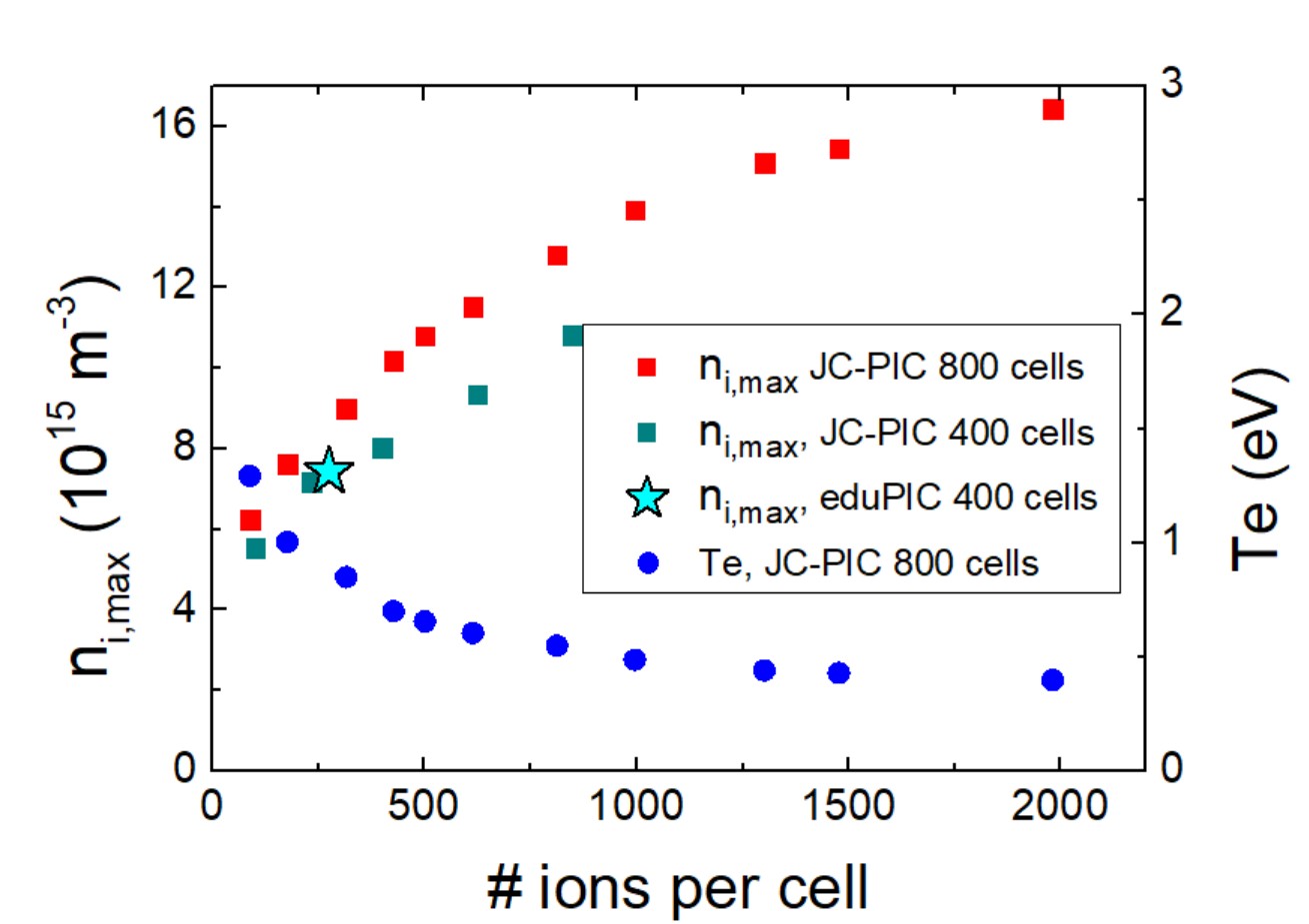
Figure 167: Maximum ion density (left axis) and central electron temperature (right axis) in the steady state, as a function of the number of ions per cell, for the 400-cell and the 800-cell simulations. The eduPIC result (400 cells ≈275 ions per cell) is also shown.

This figure contains the whole study in one plot, and it must be read carefully.

Consider first the 800-cell series. The density increases steadily with the particle number, from about 7×10¹⁵ m⁻³ at one hundred ions per cell to twice that value at two thousand ions per cell. At the same time the central electron temperature decreases from about 1.9 eV to a little more than 0.5 eV. The convergence is real but slow. Even near 1000 ions per cell, which is the value of this case, the density still changes by about ten per cent when the particle number is doubled again. There is no sharp threshold above which the result becomes correct. There is a trend that becomes gradually less steep, and only an explicit variation of the particle number shows where a given run is placed on this trend.

The 400-cell series gives complementary information. It follows the 800-cell series at low particle numbers, then becomes constant early. Here the grid becomes the limiting factor. When the density increases the Debye length becomes shorter, $\Delta x / \lambda_D$ approaches unity on the coarse grid, and the smoothing by the grid limits the density that the run can reach. Refining the particle number without refining the grid, or the opposite, gives no improvement in the end. The two resolutions must be improved together.

Finally, the eduPIC [90] point is exactly on the 400-cell JC-PIC curve at its own particle number. The two codes agree completely when the numerical settings are the same. At these settings both are about a factor of two below the converged density. Reproducing a published reference case validates the code, but it does not by itself give the correct plasma. This difference is the reason for this folder.

Summary

For this discharge the number of particles per cell is a convergence parameter of its own. It has the same status as the cell size and the time step, and it must be varied explicitly. The same is true for any discharge with a trapped group of low-energy electrons that has almost no collisions. The Ramsauer minimum makes this the normal situation in argon and in the heavier rare gases [91]. The usual stability criteria do not help: $\Delta x / \lambda_D$ and $\omega_{pe} \Delta t$ have correct values in the under-resolved runs. The cost of the accurate result is the computation time. The practical solution is the checkpoint and restart mechanism, with the machine left to run during the night.

VI.C Pressure Effect — Godyak et al.

This section follows one argon capacitive discharge over three decades of gas pressure, at a fixed driving frequency and a fixed discharge current. The question is how the electrons behave. The answer is not the one that intuition suggests. Between a few mTorr and a few Torr the electron energy distribution does not simply become wider or narrower. It changes shape completely and is inverted at a threshold pressure. In an ordinary gas the mean electron energy decreases steadily as the pressure increases. Here it first decreases to an abnormally low value and then increases by a factor of five. The cause is the Ramsauer minimum of argon. The measurements that established this effect are those of Godyak, Piejak and Alexandrovich [91-92].

This case is of double interest for a particle code. It is a demanding physical benchmark, because the quantity to reproduce is the shape of a distribution function over four decades of magnitude, not a density or a current. It is also a demanding numerical benchmark, for the reason explained in the eduPIC sensitivity section. The population that produces the whole effect is a group of slow, nearly collisionless electrons trapped in the ambipolar potential well. This group is exactly the one that an under-resolved simulation destroys.

The experiment

Godyak and co-workers measured electron energy distributions in a parallel-plate RF discharge that was symmetric both geometrically and electrically. The probe system was designed specifically for the RF environment. It was RF-compensated and continuously cleaned. The signal was processed by AC modulation rather than by numerical differentiation of a fitted characteristic. This care with the probe is the reason why these data resolve the low-energy electrons at all. The classic failure of RF probe diagnostics is a smeared second derivative. This smearing suppresses precisely the slow electrons and gives a mean energy several times too large.

• Argon (and, for comparison, helium), gas pressure from 2 mTorr to 3 Torr
• Symmetric parallel-plate discharge, electrode gap L = 6.7 cm
• Driving frequency 13.56 MHz
• Discharge current density fixed at 10 A/m² (1 mA/cm²; in the simulation this value is the amplitude of the imposed RF current). The current, not the voltage, is the control parameter
• EEPF measured at the midplane of the discharge

The fixed-current condition is important and must be restated: the applied voltage is the value that the discharge requires at each pressure. JC-PIC therefore runs these cases in current-driven mode, so that the same quantity is imposed in the simulation and in the experiment. If a voltage were imposed instead, two different discharges would be compared. The resulting voltage is itself a result. At 10 A/m² the amplitude on the electrode is 160 V at 10 mTorr in argon and 94 V at 100 mTorr. In helium at 30 mTorr it is 361 V.

What the measurements show

Two figures of [92] contain the result. Figure 170 gives the family of argon EEPFs as the pressure is increased at constant current. Figure 171 gives the effective electron temperature, defined as two-thirds of the mean electron energy, for argon and for helium under identical conditions.

At the lowest pressures the argon EEPF is concave on a semi-logarithmic plot. It is not one Maxwellian but two: a large cold group at low energy and a hot, dilute tail. About nine electrons in ten belong to the cold group. Its temperature is close to the energy of the Ramsauer minimum, a few tenths of an eV. The tail is one order of magnitude hotter and contains the electrons that produce the ionization. The resulting effective temperature is abnormally low. It decreases from about 1.7 eV at 2 mTorr to a minimum near 0.65 eV between 10 and 20 mTorr. These values are far below any value that a Maxwellian description of this discharge would suggest, and far below the values reported by earlier probe measurements.

Between about 40 and 100 mTorr the situation is inverted. The effective temperature increases steeply to about 3 eV, and the EEPF becomes convex: the cold peak disappears. Above ~0.5 Torr the distribution is Druyvesteyn-like and becomes flat as the energy goes to zero. Beyond the transition the effective temperature is nearly constant, between 2.7 and 3.2 eV, up to 3 Torr.

Helium, measured in the same cell at the same current, behaves in the opposite way, and monotonically. Its effective temperature decreases from 6.4 eV at 30 mTorr to 2.3 eV at 3 Torr. This is the ordinary behaviour of a collision-dominated discharge. The anomaly is therefore not an artefact of the geometry or of the diagnostic. It is a property of the gas.

Why the Ramsauer minimum does this

In argon the electron-atom momentum-transfer cross-section has a deep minimum near 0.3 eV. It decreases by about two orders of magnitude between 10 eV and the minimum. The electron population therefore separates into two groups that hardly interact with each other.

The slow electrons are created by ionization in the centre of the discharge and are cooled into the Ramsauer energy window. Their collision frequency is so low that their mean free path is larger than the half-width of the plasma. This has two consequences. First, their oscillation in the RF field is essentially collisionless, because the square of their collision frequency is far below the square of the driving frequency. An electron that oscillates without collisions gains no energy on average, whatever the strength of the field. Second, they cannot cross the DC ambipolar potential barrier that confines them, so they never reach the oscillating sheath edges where stochastic heating takes place. They are trapped, and they remain cold. Electron–electron collisions, whose frequency is large at low temperature, make this group Maxwellian internally. For this reason the group appears as a clean straight segment on the EEPF.

The fast electrons are on the other side of the Ramsauer minimum, where the cross-section is large. They collide frequently, they cross the ambipolar barrier easily, they move back and forth between the two sheaths and are heated stochastically there, and they produce the ionization. The two groups have different temperatures, different confinement and different roles. The measured distribution is their sum.

Increasing the pressure destroys this arrangement. It does so abruptly rather than gradually, because the feedback is positive. As the pressure decreases, stochastic heating at the boundaries replaces ohmic heating in the bulk. More heating at the boundaries reduces the RF field in the plasma body, which lowers the electron energy. Since the collision frequency in argon increases with energy, a lower energy reduces the bulk ohmic heating even more. The result is a threshold rather than a gradual change. Godyak found that the transition scales as a pressure–gap product, at a few tenths of a Torr·cm in argon at 13.56 MHz. For the 6.7 cm gap of this section this gives a transition near 70 mTorr, exactly where the measured effective temperature jumps. Below the threshold the discharge is in the non-local, stochastically heated regime. The ratio of the total RF power transferred to the electrons to the collisional power computed from the measured plasma reaches 10³ at the lowest pressures. In other words, essentially none of the heating is ohmic. Above the threshold the discharge is collisional and local, the EEPF is determined by the local field, and argon behaves like any other gas.

Comparison with JC-PIC

Eleven runs were made for this comparison. All are current-driven at 10 A/m² and 13.56 MHz across the 6.7 cm gap. Argon was run at 2, 10, 50, 100 and 500 mTorr and at 1 Torr. Helium was run at 30, 50, 100 and 500 mTorr and at 1 Torr. The two highest helium pressures are the least converged of the series. The others are stationary to better than 1 % over the last fifth of their duration.

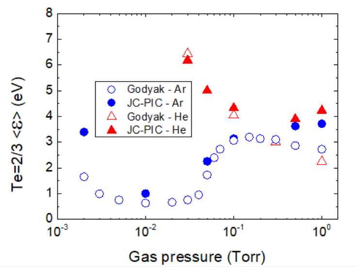
Figure 168: Effective electron temperature as a function of gas pressure at fixed current density. Open symbols: the measurements of figure 22 of [92], digitised. Filled symbols joined by a line: JC-PIC. Blue is argon, orange is helium.

Table 1: The same numbers. The effective temperature is computed from the simulated distribution at the midplane exactly as it is defined in [92], as two-thirds of the mean electron energy.

What agrees. The non-monotonic behaviour of argon is reproduced without any adjustment. The effective temperature decreases to a minimum, and the minimum is at 10 mTorr, where it is measured. Above it the temperature increases steeply and then becomes constant. At 100 mTorr, just after the transition, the agreement is quantitative: 3.14 eV against a measured value of 3.07. In the simulation as in the experiment, helium behaves in the opposite way, monotonically. At 30 mTorr the two numbers agree to 4 %, 6.18 eV against 6.44. The two gases differ by a factor of six at comparable pressure, in the code as in the experimental cell.

What does not agree. There are two systematic departures, and they are not the same one. Below 50 mTorr JC-PIC is too hot in argon by a factor of about 1.5 to 2: 1.01 eV against 0.64 at 10 mTorr, 3.40 against 1.66 at 2 mTorr. Above 500 mTorr it is too hot by about 30 %, in argon and in helium alike.

The low-pressure departure has a candidate cause that can be tested inside the code. It is the subject of the numerical warning below: the trapped cold group is destroyed by anything that scatters it, including the numerical field noise. The 10 mTorr point was run twice, with 512 cells and half a million macro-particles and with 700 cells and 1.1 million. The effective temperature decreased from 1.24 to 1.01 eV when the resolution was increased. It is still decreasing. The measured 0.64 eV may simply be further along the same curve. A second and independent contribution is the energy binning of the diagnostic itself. The distributions here are accumulated with 200 bins over 200 eV, that is one bin per eV. The whole cold group, which is at a few tenths of an eV, therefore falls in the first bin and is counted at its centre, 0.5 eV. This alone biases the effective temperature upward by about 0.1 eV at 10 mTorr. Both effects act in the same direction, and both come from the simulation, not from the discharge.

The high-pressure departure is different, because it appears in both gases and in a regime where the electrons are collisional and the simulation is easy. The most probable cause is a missing loss channel: JC-PIC has no excited-state population, so it has no stepwise ionization through metastables and no super-elastic collisions. Ionization from a metastable costs about 4 eV instead of 15.8. A code without this process must therefore have hotter electrons to sustain the same discharge, and metastables are important precisely at high pressure. This is a hypothesis and not a demonstration. However, it is consistent with the sign, with the size, and with the fact that both gases show the departure.

Figure 169: Electron energy probability function at the midplane, time-averaged, (a) in argon and (b) in helium, at the pressures of the series. To be compared with figure 20 of [92]. In argon the curve is concave at 2 and 10 mTorr, with a steep cold part and a long hot tail. It becomes convex at 500 mTorr and 1 Torr, where it bends downward and is flat at the bottom. In helium there is no such change: the shape is the same at every pressure and only the tail becomes shorter as the pressure increases.

Figure 169 is the most important part of the comparison, because it shows the shape and not only the number. At 10 mTorr, 82 % of the simulated electrons are below 2 eV. The distribution decreases by two decades between 0.5 and 5 eV, and then turns into a much flatter tail. This is the two-temperature structure of [92], with the same proportion of cold electrons as in the measurements. At 1 Torr the same discharge has a distribution that is flat at the bottom and cut off near 20 eV. Nothing was changed between the two runs except the gas density.

A numerical warning: particles per cell

JC-PIC reproduces this physics, but only when the simulation is resolved well enough. The requirement is more severe here than in an ordinary discharge. The reason is the one analysed in the eduPIC — Sensitivity / Accuracy section. With too few particles per cell, the self-consistent field contains a fluctuating component of purely numerical origin. This component acts on the electrons as a spurious scattering in velocity space [80]. The electrons affected are precisely the trapped low-energy electrons: this group is nearly collisionless and therefore has no real process that competes with the numerical one. Numerical fluctuations lift them over the ambipolar barrier. They reach the sheath edges and are really heated there. The cold peak, which is the whole signature of the low-pressure regime, disappears.

An under-resolved run at 10 mTorr therefore does not simply give a slightly wrong temperature. It can give a single-temperature distribution and an effective temperature several times too large. In other words, it reproduces the wrong regime. The 10 mTorr pair quoted above measures the effect directly. The lesson is that at this pressure the result still changes with the resolution. It is 1.24 eV with 512 cells and half a million particles, and 1.01 eV with 700 cells and 1.1 million. The remedy is a large number of particles per cell, imposed as described in the sensitivity case. The ceiling on the total number of macro-particles is set to the desired number per cell multiplied by the number of cells. A grid fine enough to resolve the Debye length at the density peak is also needed. The low-pressure cases of this section are the most demanding. They are the ones to check first when the EEPF looks too Maxwellian.

The three cases in this section

Eleven pressures were run. Three are documented here; they were chosen because together they contain the whole effect.

• Argon, 10 mTorr, 10 A/m² — deep in the non-local, stochastically heated regime, at the minimum of the measured effective temperature. The EEPF has a strong two-temperature structure and the trapped cold group dominates. This is the numerically demanding case.
• Argon, 100 mTorr, 10 A/m² — just after the transition, on the plateau. The EEPF is convex, the heating is mostly collisional, and the discharge behaves like an ordinary one.
• Helium, 30 mTorr, 10 A/m² — the control case. Same cell, same current, same frequency, a gas without a Ramsauer minimum, and a pressure lower than in the argon case. Nevertheless the discharge is heated mainly in the bulk and its electrons are six times hotter.

The three descriptions contain the same two figures, so that they can be compared side by side. The first shows the distribution and the time-averaged profiles. The second shows the ionization rate and the electron power resolved in position and time. The last of these shows the heating-mode transition most directly.

VI.C. Case 1 Argon 10 mTorr — 10 A/m²

The low-pressure, stochastically heated regime

This case is at the lowest pressure of the pressure scan of the section. It is in the regime where Godyak and co-workers measured an abnormally low electron energy [91-92]. At 10 mTorr the effective electron temperature of the argon discharge reaches its minimum, ≈0.64 eV [92]. At this pressure the two-temperature structure of the electron energy distribution is most pronounced. It is also the pressure where the simulation is most difficult to converge. The physics depends entirely on a group of slow electrons. In an under-resolved run, the only significant scattering of these electrons is numerical.

Conditions of the Simulation

• Capacitive RF discharge in argon, symmetric parallel-plate geometry
• Gas pressure 10 mTorr (1.33 Pa), gas temperature 300 K
• Gap length L = 6.7 cm
• Driving frequency 13.56 MHz
• Current-driven: RF current density amplitude 10 A/m² (1 mA/cm²); the applied voltage is the voltage required by the discharge
• Ion-induced secondary electron emission with γ = 0.1 at both electrodes (emitted at 2 eV); electrodes otherwise absorbing

Numerical resolution - 700 grid cells (Δx = 95.7 µm), time step at most 5×10⁻¹¹ s - Maximum of 1.1×10⁶ macro-particles per species, that is about 1600 per cell at the final density of the discharge - Run to 413 µs; the averaged and phase-resolved diagnostics accumulate from 50 µs onwards

The two resolution requirements are not independent, and both must be satisfied. The cell size has to resolve the Debye length at the density peak. The number of particles per cell has to be large enough that the numerical field fluctuations do not untrap the low-energy electrons. The second requirement is the limiting one at this pressure, and it is not yet fully satisfied even here. The same case run with 512 cells and half a million particles gives an effective temperature of 1.24 eV, against 1.01 eV for the run described here. The result still changes with the resolution, and it changes toward the measurement. See the eduPIC — Sensitivity / Accuracy case for the results of an under-resolved run.

Physics

At 10 mTorr the electron mean free path in the Ramsauer window is larger than the plasma half-width, so the discharge is in the non-local regime. The electron energy distribution is a function of the total energy and not of the local field. Almost all of the RF power reaches the electrons through stochastic heating at the oscillating sheath edges, and not through ohmic dissipation in the bulk.

The electron population is divided in two groups. Slow electrons, cooled to energies close to the Ramsauer minimum near 0.3 eV, collide so rarely that their oscillation in the RF field is collisionless and gives them no energy. They cannot cross the DC ambipolar barrier, so they never reach the sheath edges where the heating occurs. They accumulate as a cold, dense, trapped group. Fast electrons, on the high-energy side of the minimum, collide often. They cross the barrier freely, move back and forth between the sheaths, are heated there, and produce the ionization. The measured distribution is the sum of the two groups. It is concave on a semi-logarithmic plot. The resulting low effective temperature is simply the average of a large cold population and a small hot one.

The converged state

• Effective electron temperature at the midplane 1.01 eV, against the measured 0.64 eV [92]
• Mean electron energy at the midplane 1.42 eV; 82 % of the electrons are below 2 eV
• Peak ion density 2.84×10¹⁵ m⁻³, at the centre of the gap
• Time-averaged plasma potential 77 V; voltage amplitude on the electrode 160 V; DC self-bias 0.2 V, that is zero as symmetry requires
• Sheath width 0.64 cm, ion flux to each electrode 1.07×10¹⁸ m⁻²s⁻¹
• Power given to the electrons 13.5 W/m², of which 76 % in the outer fifth of the gap

Results

Figure 172: (a) Electron energy probability function at the midplane, time-averaged, for two resolutions of the same case. A higher resolution lowers the tail and therefore the effective temperature, from 1.24 to 1.01 eV. The shape is the concave, two-temperature shape of figure 20 of [92]: a steep decrease of two decades between 0.5 and 5 eV, then a much flatter tail. (b) Time-averaged ion and electron densities, and the time-averaged potential on the right axis. The plateau of this potential across the bulk is the ambipolar barrier that traps the cold group.

Figure 173: Spatio-temporal maps over one RF period (73.7 ns), position on the horizontal axis and time on the vertical axis, of (a) the ionization rate and (b) the electron power $\mathbf{j}\cdot\mathbf{E}$. Produced with the JC-PIC (x,t) viewer.

These two maps are the direct picture of non-local, stochastic heating. The ionization does not follow the field. It is produced by beams that leave each sheath while it expands and cross the whole 6.7 cm gap in a straight line. These beams produce their ionization far from the place where they were accelerated. The power map is almost empty between the sheaths. The energy is given to the electrons in two bright spots per period, one at each sheath edge during its expansion. In the central three-fifths of the gap the cycle-averaged power is not only small but negative, −21 W/m³: the electrons give energy back to the field there. This is the signature of the regime. The comparison with the 100 mTorr case, where the same quantity is positive and ten times larger, is the purpose of this pair of descriptions.

VI.C. Case 2 Argon 100 mTorr — 10 A/m²

Just past the heating-mode transition

This case is the companion of the 10 mTorr case and its opposite. The pressure has been increased by a factor of ten, and everything else is unchanged. The discharge has crossed the heating-mode transition. The measured effective electron temperature has increased from ≈0.64 eV to ≈3.07 eV, and the electron energy distribution has changed from concave to convex [92]. The pair 10 / 100 mTorr therefore covers the whole effect, and the comparison between the two descriptions is the purpose of the section.

Conditions of the Simulation

• Capacitive RF discharge in argon, symmetric parallel-plate geometry
• Gas pressure 100 mTorr (13.3 Pa), gas temperature 300 K
• Gap length L = 6.7 cm
• Driving frequency 13.56 MHz
• Current-driven: RF current density amplitude 10 A/m² (1 mA/cm²); the applied voltage is the voltage required by the discharge
• Ion-induced secondary electron emission with γ = 0.1 at both electrodes (emitted at 2 eV); electrodes otherwise absorbing

Numerical resolution - 512 grid cells (Δx = 131 µm), time step at most 5×10⁻¹¹ s - Maximum of 5×10⁵ macro-particles per species, that is about 1000 per cell - Run to 369 µs; the averaged and phase-resolved diagnostics accumulate from 50 µs onwards

This case is less demanding than the 10 mTorr case, because the electrons on which it depends are collisional. There is a real scattering process that competes with the numerical one, so the distribution is much less sensitive to a moderate number of particles. This is visible in the result: this is the point of the whole series where JC-PIC and the measurement agree best.

Physics

At 100 mTorr the discharge has crossed the threshold. Godyak located this threshold at a pressure–gap product of a few tenths of a Torr·cm in argon at 13.56 MHz [91], that is near 70 mTorr for this 6.7 cm gap. Ohmic heating in the bulk now dominates over stochastic heating at the sheath edges. The electron mean free path has become smaller than the plasma half-width, and the distribution is determined by the local field and not by the total energy.

The trapped cold group has disappeared, and with it the two-temperature structure. The distribution is convex and tends toward a Druyvesteyn shape. Above roughly 0.5 Torr it becomes flat as the energy goes to zero. This is the opposite of the low-pressure peak, and it is again a consequence of the Ramsauer minimum. A cross-section that increases with energy lets the slowest electrons accelerate almost freely, so it empties the bottom of the distribution instead of filling it.

The transition between the two cases is abrupt and not gradual. The reason is a positive feedback. More stochastic heating at the boundaries reduces the RF field in the plasma body. A lower field means a lower electron energy. Because the collision frequency in argon increases with energy, a lower energy reduces the bulk ohmic heating even more. Each effect reinforces the next, so the discharge does not pass smoothly from one mode to the other: it switches.

The converged state

• Effective electron temperature at the midplane 3.14 eV, against the measured 3.07 eV [92]; the difference is 2 %
• Mean electron energy at the midplane 4.67 eV; 20 % of the electrons are below 2 eV, against 82 % at 10 mTorr
• Peak ion density 2.06×10¹⁵ m⁻³
• Time-averaged plasma potential 50 V; voltage amplitude on the electrode 94 V, against 160 V at 10 mTorr for the same current; DC self-bias −0.2 V
• Sheath width 0.35 cm, ion flux to each electrode 7.2×10¹⁷ m⁻²s⁻¹
• Power given to the electrons 30.9 W/m², of which 10.6 W/m² (an average of 265 W/m³, read on the (x,t) map) in the central three-fifths of the gap

Results

Figure 174: (a) Electron energy probability function at the midplane, time-averaged, with the 10 mTorr case of the companion description on the same axes. The contrast is the main result of the section: concave at 10 mTorr, convex at 100 mTorr, in the same reactor at the same current. To be compared with figure 20 of [92]. (b) Time-averaged ion and electron densities, and the time-averaged potential on the right axis.

Figure 175: Spatio-temporal maps over one RF period (73.7 ns) of (a) the ionization rate and (b) the electron power $\mathbf{j}\cdot\mathbf{E}$, on the same axes as figure 175 of the 10 mTorr description.

Both maps have changed character. The ionization no longer travels. It is produced in two compact spots next to the sheaths, where the electrons are accelerated, and it stays there. The beams that crossed the whole gap at 10 mTorr have disappeared, because at ten times the gas density an electron can no longer cross the gap without a collision. The power map is no longer empty in the middle. A broad region of positive cycle-averaged power now covers the whole bulk, +265 W/m³ on average against −21 W/m³ at 10 mTorr. This change of sign, in one number, is the heating-mode transition.

VI.C. Case 3 Helium 30 mTorr — 10 A/m²

The control: a gas without a Ramsauer minimum

The two argon cases of this section show a discharge in which the electrons behave in an unusual way at low pressure. The question is whether this behaviour comes from the discharge or from the gas. If it came from the discharge, any capacitive discharge at a few tens of mTorr in a 6.7 cm gap would do the same [91-92]. Godyak answered this question by measuring helium in the same cell, at the same current and the same frequency. This case reproduces that control measurement [92].

Helium has no Ramsauer minimum. Its momentum-transfer cross-section is smooth and almost constant at low energy, and it does not fall sharply near 0.3 eV. There is therefore no energy range in which slow electrons collide very little. Helium should then behave as an ordinary gas at every pressure: an effective temperature that decreases monotonically when the pressure increases, no two-temperature structure, and heating spread through the bulk. This is what is measured, and this is what JC-PIC gives.

The pressure used here, 30 mTorr, is the lowest pressure at which helium was measured in [92], and it is higher than the pressure of the 10 mTorr argon case. The comparison is therefore conservative. If the unusual behaviour were caused by the pressure, helium at 30 mTorr would be closer to the normal behaviour than argon at 10 mTorr for this reason alone. This is not the case: the two discharges do not follow the same curve at all.

Conditions of the Simulation

• Capacitive RF discharge in helium, symmetric parallel-plate geometry
• Gas pressure 30 mTorr (4.0 Pa), gas temperature 300 K
• Gap length L = 6.7 cm
• Driving frequency 13.56 MHz
• Current-driven: RF current density amplitude 10 A/m², the applied voltage being the voltage required by the discharge
• Ion-induced secondary electron emission with γ = 0.35 at both electrodes (emitted at 2 eV); the electrodes are absorbing for the other particles

Numerical resolution - 256 grid cells (Δx = 262 µm), time step at most 5×10⁻¹¹ s - Upper limit of 5×10⁵ macro-particles per species, that is about 2000 per cell at the density reached by the discharge. The density here is ten times lower than in argon, so the same limit gives a much finer sampling - Run to 67 µs, with the diagnostics accumulated from 50 µs onwards. This run is shorter than the argon runs and is the least converged of the series. The density was constant to better than 0.5 % over the last third of the run. The numbers below should be considered accurate to a few percent rather than to one percent.

The converged state

• Effective electron temperature at the midplane 6.18 eV, against the measured value 6.44 eV [92], a difference of 4 %
• Mean electron energy at the midplane 9.34 eV, against 1.42 eV in argon at 10 mTorr
• Peak ion density 2.74×10¹⁴ m⁻³, ten times lower than in argon at the same current
• Time-averaged plasma potential 179 V. Voltage amplitude on the electrode 361 V, against 160 V in argon
• Ion flux to each electrode 1.56×10¹⁸ m⁻²s⁻¹, larger than in argon although the density is much lower, because the helium ion is light
• Power given to the electrons 60.9 W/m², of which 60 % in the central three-fifths of the gap

Results

Figure 176: (a) Time-averaged electron energy probability function at the midplane, with the argon case at 10 mTorr on the same axes. Helium gives a single distribution with one slope over three decades. Argon, at a lower pressure, gives the two-temperature curve, with 82 % of its electrons below 2 eV. (b) Time-averaged ion and electron densities, and the mean electron energy on the right axis. The energy is high everywhere and increases toward the electrodes. There is no group of cold electrons in the middle.

Figure 177: Spatio-temporal maps over one RF period (73.7 ns) of (a) the ionization rate and (b) the electron power $\mathbf{j}\cdot\mathbf{E}$, on the same axes as the two argon cases.

The power map is the map to compare. In argon at 10 mTorr, three quarters of the energy is given to the electrons in two regions at the sheath edges, and the bulk loses energy. Here, at three times this pressure, 60 % of the power is given in the bulk, and the value averaged over the cycle is +904 W/m³ there. This value is forty times the argon value and it has the opposite sign. The heating mode is not fixed by the pressure, by the gap or by the frequency, which are identical in the two runs. It is fixed by the gas.

VI.C. Case 4 ascii

VI.D Dual-Frequency RF Discharges and the Electrical Asymmetry Effect

A central limitation of single-frequency capacitively coupled RF processing is that the ion flux and the ion bombarding energy are coupled. When the voltage is increased to increase the flux, the ion energy also increases. The ion flux sets the process throughput, and the ion energy controls the etching and deposition chemistry. For this reason, independent control of the two quantities is very desirable, above all in microelectronics, where silicon wafers are processed. Two routes to this independent control are studied in this chapter. The present section covers the electrical route.

Dual-frequency operation

The classical approach, introduced in the 1990s, superimposes two RF voltages of very different frequencies. The heavy ions can partly follow the low-frequency component. This component therefore mainly controls the ion bombarding energy through the sheath voltage. The high-frequency component controls the plasma density and therefore the ion flux. Using PIC simulations, Boyle et al. [101] showed that this decoupling is efficient when the ratio of the low to the high frequency is below about 0.1. A disadvantage is that the two frequencies are not perfectly independent (frequency coupling). This limits the range of separate control that can be obtained.

The Electrical Asymmetry Effect (EAE)

A different route, proposed by Heil et al. [93], uses instead the phase between two harmonically related frequencies. If a temporally symmetric voltage waveform contains an even harmonic of its fundamental, the sheaths in front of the two electrodes are necessarily asymmetric. A DC self-bias then develops, even in a geometrically symmetric reactor. The simplest realization combines the fundamental and its second harmonic:

with f = 13.56 MHz and a phase shift θ applied to the fundamental. The resulting self-bias is given by a symmetry parameter ε together with the extreme (most positive and most negative) values of the applied waveform. The parameter ε is the ratio of the maximum voltages that the two sheaths can sustain. It is equal to unity for identical electrodes:

These extreme values depend on θ. The self-bias, and therefore the ion energy, can thus be adjusted continuously by the phase alone, at almost constant amplitude, frequency and absorbed power. The self-bias is a nearly linear function of θ. It takes its largest values, with opposite polarities, near θ = 0° and θ = 90°. It passes through zero near θ = 45°, where the waveform becomes symmetric and the discharge behaves symmetrically.

PIC verification (Donkó et al., 2009)

Donkó et al. [94] verified the EAE with a particle-in-cell simulation of a geometrically symmetric dual-frequency argon discharge driven at 13.56 and 27.12 MHz. When the phase is scanned, the DC self-bias reaches about 70% of the amplitude of each harmonic (≈ ±215 V for 315 V). The ion flux to each electrode remains constant to within a few percent. The maximum ion energy at a given electrode changes by a factor of about three. The electrical roles of the two electrodes can be reversed simply by changing the phase.

The cases in this section

The four cases reproduce, with JC-PIC, the phase scan of Donkó et al. [94] at 20 mTorr with a 6.7 cm gap (argon, V₀ = 315 V), for phase shifts of 0°, 45°, 60° and 90°. The central illustration is the energy distribution of the ion flux (IFEDF) at both electrodes. When θ is varied, the IFEDFs of the grounded and the powered electrode move apart and exchange their positions. This shows the adjustable, mirror-imaged ion energies, while the integrated ion flux to each electrode remains nearly constant. In JC-PIC the DC self-bias is obtained physically, by inserting a blocking capacitor between the voltage source and the discharge.

VI.D. Case 1 Electrical Asymmetry Effect — Phase shift θ = 90°

At θ = 90° the applied waveform 315[cos(2πf₁t + 90°) + cos(2πf₂t)] reaches the second extreme of the phase scan: the self-bias is again maximal, but with the opposite polarity to θ = 0°. The electrical roles of the two electrodes are now completely reversed. The grounded electrode is behind the thicker sheath and collects the more energetic ions, while the powered electrode collects the less energetic ones. This case is the mirror image of θ = 0°. Together, the two cases define the full range of ion-energy control. In JC-PIC the powered electrode is the left one (x = 0) and the grounded electrode the right one (x = L). The two electrodes are geometrically identical and have the same secondary-emission coefficient, so every asymmetry reported below is produced by the phase alone.

Conditions of the Simulation

Dual-frequency capacitive RF discharge (geometrically symmetric) Argon, p = 20 mTorr (≈2.67 Pa, Tg = 350 K, N = 5.52×10²⁰ m⁻³) Gap length L = 6.7 cm Applied voltage V(t) = 315 [cos(2πf₁t + θ) + cos(2πf₂t)] V, with f₁ = 13.56 MHz, f₂ = 27.12 MHz Phase shift θ = 90° Secondary emission coefficient γ = 0.1 (both electrodes); electron reflection coefficient α = 0.2 DC self-bias obtained self-consistently through a series blocking capacitor Numerical parameters: Plasma density (initial) 2×10¹⁴ m⁻³ Number of grid points 1024 Particles per cell ≈ 118 Time step 2×10⁻¹¹ s Run to ≈250 μs; all the diagnostics below are accumulated from 100 μs onwards Resolution check: At the density maximum (1.9×10¹⁶ m⁻³, Te ≈ 2 eV) the Debye length is 75 μm against a cell size of 65 μm, and ωₚₑΔt ≈ 0.16. Both standard PIC criteria are satisfied, with a larger margin inside the sheaths where the density is lower. Collisionality: The electron mean free path is 3.4 cm, of the order of the gap itself, so the electrons are non-local. For the ions the mean free path is 3.7 mm for charge exchange and 1.5 mm for all ion–neutral collisions, against time-averaged sheaths of 4 to 7 mm. The sheaths are collisional, and this determines the shape of the ion energy distributions below.

Results

All the figures below come from the same run. The (x, t) maps are phase-resolved over one period of the 13.56 MHz fundamental and averaged over many cycles, so a single map describes the whole steady state.

Driving waveform and DC self-bias

Figure 178: Potential of the powered electrode (blue, left axis) and total current density (red, right axis), phase-resolved over one 13.56 MHz period (73.7 ns). The green dash-dotted line marks the DC self-bias.

The source waveform alone varies between −630 V and +354 V. Adding the second harmonic with a 90° phase makes its two excursions strongly unequal, and this inequality is the whole mechanism. The blocking capacitor charges until the electron charge and the ion charge collected per period balance at each electrode. This happens here at a self-bias of +206 V, i.e. +0.65 of the amplitude V₀ = 315 V. The electrode potential therefore goes from −424 V to +560 V. Its shallow local minimum near t = 55 ns touches the self-bias line exactly, as required by the analytical waveform. Donkó et al. [94] obtain +215 V at this phase and −213 V at θ = 0°; JC-PIC gives +206 V here and −212.5 V at θ = 0°. The agreement is better than 5%, and 0.2% at θ = 0°. The comparison also validates the model of the effect. With a symmetry parameter ε = 1, the formula of Heil et al. [93] would predict only ∓138 V. The additional bias comes entirely from the departure of ε from unity. Inverting the formula with the measured value gives ε ≈ 1.32, against ε ≈ 1.33 read from the PIC curve of figure 5 of [94]. The two sheaths are therefore not equivalent, even though the electrodes are: the mean ion density is higher in the sheath at the powered electrode. This self-amplification of the asymmetry is reproduced quantitatively. The current density (±65 A/m²) is essentially the displacement current. The fast oscillations that it carries between 25 and 35 ns are not noise. They are the plasma series resonance, excited by the non-linear charge–voltage relation of the expanding sheath. Donkó et al. report the same signature at the grounded electrode between 20 and 40 ns at θ = 90° (and at the powered electrode between 0 and 20 ns at θ = 0°). This was the first observation of the PSR in a geometrically symmetric discharge. It is possible precisely because the EAE makes the discharge electrically asymmetric.

Ion flux-energy distributions — the central result

Figure 179: Ion flux-energy distribution at the powered electrode (Left, red) and at the grounded electrode (Right, blue), accumulated from 100 μs. Each curve is normalised to unit integral, so their relative heights give no information on the flux.

This is the central figure of the case, and the direct counterpart of the ion-energy distributions of Donkó et al. [94]. The two distributions are completely separated. The ions reaching the powered electrode stop at 130 eV; those reaching the grounded electrode extend to 353 eV. The ratio is 2.7, which is the factor of about three reported in the paper. In mean energy the contrast is 80 eV against 202 eV. At θ = 0° the two curves are exchanged, and at θ = 45° they nearly coincide. Both distributions show the signature of a collisional sheath. A large fraction of the ions undergo charge exchange on their way to the electrode. Each of these ions restarts from rest at the local potential and arrives with only part of the full sheath voltage. This fills the whole energy range below the main peak. At the grounded electrode, where the sheath is thick, this gives the broad and almost flat continuum that carries roughly two thirds of the flux. At the powered electrode, where the sheath is thinner, it gives a series of resolved peaks about 25 eV apart. The peaks come from the fact that the sheath voltage is not sinusoidal: the fundamental and its second harmonic give it several extrema per period. The charge-exchange ions therefore arrive in well-defined energy groups, not as a continuum without structure. The narrow double peak at the end of each distribution (near 102 and 114 eV on the left, 306 and 327 eV on the right) is the classical bimodal, or saddle, RF structure. Ions that cross the sheath in a time comparable to the RF period see the oscillating sheath voltage and accumulate at the two turning points of the modulation. Finally, and this is the main point of the whole chapter: the energy-integrated fluxes at the two electrodes differ by only 9%, while their energies differ by a factor 2.7. In absolute terms the ions reach the two walls at a total rate of 1.5×10¹⁹ m⁻²s⁻¹, that is ≈7.6×10¹⁴ cm⁻²s⁻¹ at each electrode, against ≈9×10¹⁴ cm⁻²s⁻¹ in figure 8 of [94]. Energy and flux are indeed decoupled.

Time-averaged plasma structure

Figure 180: Time-averaged electron (cyan) and ion (blue) densities, left axis, and electric field (red), right axis, at t = 245 μs.

The plasma is asymmetric although the reactor is not. The density reaches its maximum of 1.9×10¹⁶ m⁻³ slightly to the right of the mid-plane. Donkó et al. report 1.7×10¹⁶ m⁻³ at the discharge centre, essentially independent of θ. The sheath is about 0.45 cm wide at the powered electrode and about 0.7 cm at the grounded one. The field at the wall is correspondingly larger on the grounded side. In both sheaths the ion density remains where the electron density has already fallen to zero, which is what makes them sheaths. The field remains essentially zero across the quasi-neutral bulk. The two ratios can be checked against each other. A Child-law sheath scales as V^(3/4), so the mean sheath voltages deduced from the IFEDF (ratio 2.7) would give a thickness ratio of 2.1, against 1.6 measured. The remaining difference comes from the densities at the two sheath edges, which are not equal. This is the same effect that makes ε depart from unity in Figure 178.

Electron power absorption and ionization dynamics

Figure 181: Electron power absorption density in the (x, t) plane, phase-resolved over one 13.56 MHz period and averaged over many cycles. Red is heating, blue is cooling.

Power is absorbed almost entirely at the two sheath edges, in the classical alternation of heating during sheath expansion and cooling during sheath collapse. The strongest event, of order 2.5×10⁵ W/m³, occurs at the grounded sheath edge between 20 and 35 ns. This is just after the electrode potential has passed its minimum and the grounded sheath starts to expand. The corresponding event at the powered electrode, between 0 and 18 ns, is clearly weaker. This is exactly the map of figure 9 of [94]. There, most of the electron power is dissipated at the grounded electrode at θ = 90° and at the powered one at θ = 0°. The peak level is the same (2.9×10⁵ W/m³ there). Inside this heating event there is a series of separate hot spots instead of a single one. This is again the plasma series resonance, the same oscillation seen on the current of Figure 178. The asymmetry of the electron heating is the dynamical counterpart of the asymmetry of the ion energies, and both follow from the same self-bias.

Figure 182: Ionization rate in the (x, t) plane over one low-frequency period.

The expanding sheaths launch beams of energetic electrons that cross the gap and ionize on their way; these are the diagonal streaks. The dominant beam leaves the grounded sheath edge at t ≈ 25 ns. Its leading edge covers 3.9 cm in 14 ns, that is 2.8×10⁶ m/s or about 22 eV, just above the 15.8 eV ionization threshold of argon. This is exactly the population that makes the streak visible. The peak rate, 1.3×10²¹ m⁻³s⁻¹, is reached in the first millimetres of this beam. A weaker beam leaves the powered sheath at t ≈ 5 ns and another at t ≈ 48 ns. The second harmonic gives two expansion events per low-frequency period at each electrode, but of very unequal strength.

Figure 183: Mean electron energy in the (x, t) plane over one low-frequency period.

The colour scale is set by the sheaths, where the mean energy reaches 200 to 250 eV. These are the secondary electrons emitted under ion impact and accelerated across the full sheath voltage, together with the tail of the bulk electrons that can penetrate the sheath. The bulk itself is near 3 eV (Te ≈ 2 eV) and appears uniformly dark. The map is a direct picture of the sheath motion. At the grounded electrode the high-energy region is present over almost the whole period and only becomes thinner around t = 20 ns. At the powered electrode it exists only between t ≈ 8 and 32 ns, and it is brightest when the electrode potential is most negative. Secondary electrons are not a detail here. They are released at 1.4×10¹⁸ m⁻²s⁻¹, against 1.8×10¹⁹ m⁻²s⁻¹ of volume ionization, that is 8% of the electron production. But each of them is accelerated through the whole sheath voltage, so their contribution to the ionization itself is much larger than this figure suggests.

What this case demonstrates

At fixed voltage amplitude and fixed frequencies, a single phase angle changes the maximum ion bombarding energy at a given electrode by a factor 2.7 and its mean by 2.5. This follows by mirror symmetry with θ = 0°, where the two curves of Figure 179 are exchanged. At the same time the ion flux stays within a few percent, and the total absorbed power, according to [94], within 6%. This is the electrical asymmetry effect. It is important industrially for this reason: in a wafer-processing reactor the throughput, which is set by the flux, and the surface chemistry, which is set by the energy, become independent controls. The θ = 90° case is at one end of the scan. The θ = 0° case is at the other end, with the roles of the electrodes exchanged. The θ = 45° case is in the middle, where the discharge is nearly symmetric. The four cases together cover the whole control range.

VI.D. Case 2 Electrical Asymmetry Effect — Phase shift θ = 60°

θ = 60° is an intermediate point of the scan. It is after the sign change of the self-bias and before the extreme case θ = 90°. This case shows that the effect can be adjusted continuously and not only switched on or off: the self-bias is positive but moderate, the two ion energy distributions are separated but still overlap, and the electron heating is shared almost equally between the two sheaths.

Conditions of the Simulation

Dual-frequency capacitive RF discharge (geometrically symmetric) Argon, p = 20 mTorr (≈2.67 Pa, Tg = 350 K, N = 5.52×10²⁰ m⁻³) Gap length L = 6.7 cm Applied voltage V(t) = 315 [cos(2πf₁t + θ) + cos(2πf₂t)] V, with f₁ = 13.56 MHz, f₂ = 27.12 MHz Phase shift θ = 60° Secondary emission coefficient γ = 0.1 (both electrodes); electron reflection coefficient α = 0.2 DC self-bias obtained self-consistently through a series blocking capacitor Numerical parameters: Number of grid points 1024, ≈118 particles per cell, time step 2×10⁻¹¹ s Diagnostics accumulated from 100 μs onwards In JC-PIC the powered electrode is the left one (x = 0) and the grounded electrode is the right one (x = L). The two electrodes are geometrically identical, so every asymmetry described below is produced by the phase alone.

Results

Figure 184: Potential of the powered electrode (blue, left axis) and total current density (red, right axis) over one 13.56 MHz period. The green dash-dotted line marks the DC self-bias.

The self-bias reaches +66.9 V. This is a third of its value at θ = 90°, and its sign is opposite to the sign at θ = 0°: the self-bias has changed sign. Inverting the model of Heil et al. [93] gives a symmetry parameter ε ≈ 1.07, compared with ε ≈ 1.06 read from the PIC curve of figure 5 of [94]. Together with the three other cases, JC-PIC reproduces the whole ε(θ) curve of [94] to within about 2%. This is the real content of the electrical asymmetry effect: the sheath densities amplify the asymmetry imposed by the waveform.

Figure 185: Ion flux-energy distribution at the powered electrode (Left, red) and at the grounded electrode (Right, blue). Each curve is normalised to unit integral.

The two distributions are clearly separated but they still overlap. The distribution at the powered electrode ends at 198 eV (mean 121 eV), and the distribution at the grounded electrode ends at 274 eV (mean 160 eV). The ratio is 1.4, compared with 2.7 at θ = 90°. Their charge-exchange structures now overlap over most of the energy range, and each distribution keeps its bimodal peak just below its own cut-off energy. This shows a continuous control: any intermediate ion energy can be obtained, not only the two extremes. The energy-integrated fluxes at the two electrodes are equal to within 0.1% here. This is the best balance of the four phases. It also shows that the flux gives no information about which electrode receives the energetic ions.

Figure 186: Electron power absorption density in the (x, t) plane over one 13.56 MHz period. Red is heating, blue is cooling.

The two heating events at sheath expansion now reach comparable levels, close to 2×10⁵ W/m³ at each electrode. At θ = 90° the grounded side was clearly dominant. Inside the event at the grounded sheath edge, between 25 and 35 ns, there is a series of separate hot spots. This is the plasma series resonance, the same oscillation that appears in the current of Figure 184.

What this case shows

Between the two extremes the effect is continuous and monotonic. The intermediate phases are what make the effect useful: the maximum ion energy at a given electrode can be set anywhere between about 130 and 350 eV by the phase alone. At the same time the flux remains constant to within a few percent, and the absorbed power, according to [94], to within 6%.

VI.D. Case 3 Electrical Asymmetry Effect — Phase shift θ = 45°

At θ = 45° the applied waveform 315[cos(2πf₁t + 45°) + cos(2πf₂t)] is exactly antisymmetric. Its most positive and most negative values have the same magnitude, ±554.5 V. The analytical model of Heil et al. [93] assumes two identical sheaths (ε = 1). It therefore predicts zero self-bias here. This phase is the natural mid-point of the scan. It is the point where the two electrodes should be electrically equivalent and where the bias changes sign. It is also the case where the difference between the model and the simulation is the most instructive.

Conditions of the Simulation

Dual-frequency capacitive RF discharge (geometrically symmetric) Argon, p = 20 mTorr (≈2.67 Pa, Tg = 350 K, N = 5.52×10²⁰ m⁻³) Gap length L = 6.7 cm Applied voltage V(t) = 315 [cos(2πf₁t + θ) + cos(2πf₂t)] V, with f₁ = 13.56 MHz, f₂ = 27.12 MHz Phase shift θ = 45° Secondary emission coefficient γ = 0.1 (both electrodes); electron reflection coefficient α = 0.2 DC self-bias obtained self-consistently through a series blocking capacitor Numerical parameters: Number of grid points 1024, ≈118 particles per cell, time step 2×10⁻¹¹ s Diagnostics accumulated from 50 μs onwards In JC-PIC the powered electrode is the left one (x = 0) and the grounded electrode is the right one (x = L). The two electrodes are geometrically identical, so every asymmetry described below is produced by the phase alone.

Results

Figure 187: Potential of the powered electrode (blue, left axis) and total current density (red, right axis) over one 13.56 MHz period. The green dash-dotted line marks the DC self-bias.

For an exactly antisymmetric waveform, JC-PIC gives a self-bias of −20.6 V. This value is small, as expected, but it is not zero, and it is negative. This residual value is the interesting part of this case. A symmetric waveform does not by itself produce a symmetric discharge. The bias is zero only if the two sheaths can sustain the same voltage, that is, if the symmetry parameter ε of [93] is equal to unity. Inverting the model with the measured bias gives ε ≈ 0.93 here, compared with ε ≈ 0.95 read from the PIC curve of figure 5 of [94]. Since ε < 1, the sheath at the powered electrode is still slightly the stronger one, and a small negative bias remains. Over the whole scan, the self-bias crosses zero at θ ≈ 48° in JC-PIC and not at 45°. Donkó et al. find the same kind of shift. Their PIC extremes are at 7.5° and 97.5° instead of 0° and 90°, so their zero crossing is near 52°. They note that this shift is absent from both the analytical and the fluid models. They suggest a kinetic origin, which they do not identify. JC-PIC, a completely independent code, reproduces a shift of the same sign and magnitude. This is useful evidence that the effect is real and not an artefact of one implementation.

Figure 188: Ion flux-energy distribution at the powered electrode (Left) and at the grounded electrode (Right). The two colours are swapped with respect to the other cases of this section: here Left is blue and Right is red. Each curve is normalised to unit integral.

The consequence of the residual bias is directly visible in the ion energies. The two distributions are nearly superposed, as expected at the mid-point. The cut-offs are 242 eV at the powered electrode and 227 eV at the grounded one, and the mean energies are 145 and 134 eV. However, they are still in the same order as at θ = 0°, not yet reversed: the powered electrode keeps the slightly more energetic ions. Their charge-exchange structures overlap almost completely below 180 eV. Each distribution ends with its own bimodal RF peak, at 234 eV and 199 eV respectively. The energy-integrated fluxes at the two electrodes differ by 3.6%. This is within the ±5% range that [94] gives for the whole phase scan.

Figure 189: Electron power absorption density in the (x, t) plane over one 13.56 MHz period. Red is heating, blue is cooling.

The near-symmetry does not extend to the electron heating. The strongest expansion event, close to 2.5×10⁵ W/m³, still belongs to the powered sheath between 0 and 18 ns. The grounded sheath produces two weaker events at about 1.5×10⁵ W/m³. The series of separate hot spots inside the first event is the plasma series resonance. Even at the phase where the ion energies almost coincide, the discharge remains measurably asymmetric. This is exactly what the residual −20.6 V of Figure 187 indicates. The time-averaged profile at the end of the run agrees with this. The sheath is 0.71 cm at the powered electrode and 0.62 cm at the grounded one. The bulk density is 1.4×10¹⁶ m⁻³ and the electron temperature is 2.0 eV at the centre.

What this case shows

The mid-point of the scan is where the analytical model is least reliable, and there is a physical reason for this. A waveform that is symmetric in theory still leaves a small self-bias, because the plasma itself determines how much voltage each sheath can hold. The phase at which the bias really becomes zero is shifted by a few degrees, in JC-PIC as in [94]. This is a kinetic effect that neither the analytical nor the fluid description reproduces.

VI.D. Case 4 Electrical Asymmetry Effect — Phase shift θ = 0°

At θ = 0° the applied waveform 315[cos(2πf₁t) + cos(2πf₂t)] is at the first extreme of the phase scan. Its positive maximum (+630 V) is much larger than its negative minimum (−354 V), so the discharge produces the largest negative self-bias of the whole scan. The powered electrode is then behind the thicker sheath and collects the energetic ions, while the grounded electrode collects the slow ions. This case and the case θ = 90°, where the two electrodes are exchanged, give the two limits of the ion-energy control.

Conditions of the Simulation

Dual-frequency capacitive RF discharge (geometrically symmetric) Argon, p = 20 mTorr (≈2.67 Pa, Tg = 350 K, N = 5.52×10²⁰ m⁻³) Gap length L = 6.7 cm Applied voltage V(t) = 315 [cos(2πf₁t + θ) + cos(2πf₂t)] V, with f₁ = 13.56 MHz, f₂ = 27.12 MHz Phase shift θ = 0° Secondary emission coefficient γ = 0.1 (both electrodes). Electron reflection coefficient α = 0.2 The DC self-bias is obtained self-consistently through a series blocking capacitor Numerical parameters: Number of grid points 1024, about 118 particles per cell, time step 2×10⁻¹¹ s Diagnostics are accumulated from 100 μs onwards In JC-PIC the powered electrode is the left one (x = 0) and the grounded electrode is the right one (x = L). The two electrodes are geometrically identical, so every asymmetry described below is produced by the phase alone.

Results

Figure 190: Potential of the powered electrode (blue, left axis) and total current density (red, right axis) during one 13.56 MHz period. The green dash-dotted line shows the DC self-bias.

The blocking capacitor reaches a self-bias of −212.5 V. This is −0.67 times the amplitude V₀ = 315 V. It is the most direct quantitative check available in this chapter. Donkó et al. [94] report a self-bias of 213 V for exactly this phase and these conditions, so the agreement is 0.2%. Inverting the model of Heil et al. [93] with the measured bias gives a symmetry parameter ε ≈ 0.74, against ε ≈ 0.74 read on the PIC curve of figure 5 of [94]. The model with ε = 1 would give only −138 V. About one third of the bias therefore comes from the self-amplification of the asymmetry by the sheath densities. The fast oscillations of the current between 0 and 15 ns are the plasma series resonance. It is excited here at the powered electrode during the expansion of its sheath. This is the mirror image of what happens at the grounded electrode at θ = 90°, and it is the same signature as the one reported in [94].

Figure 191: Ion flux-energy distribution at the powered electrode (Left, red) and at the grounded electrode (Right, blue). Each curve is normalised so that its integral is equal to one.

Compared with θ = 90°, the two curves are simply exchanged. The powered electrode now receives ions up to 353 eV (mean 201 eV), and the grounded electrode only up to 130 eV (mean 79 eV). At θ = 90° the values were 130 and 353 eV, in the opposite order. The cut-off energies agree to better than the width of one bin. This is a strong internal consistency check for the whole scan: the discharge is mirror-symmetric under θ → 90° − θ. The structures are the same as those described for θ = 90°. A charge-exchange continuum fills the range below the main peak. The local maxima at low energy are also attributed to charge exchange in the sheath by [94]. Each distribution ends with the bimodal RF saddle. The energy-integrated fluxes differ by 8% between the two electrodes.

Figure 192: Time-averaged electron (cyan) and ion (blue) densities, left axis, and electric field (red), right axis.

The maximum density is 1.65×10¹⁶ m⁻³. It is close to the 1.7×10¹⁶ m⁻³ that [94] obtains at the discharge centre, and it is also close to the value at every other phase. The density stays the same while the ion energies change. The sheath at the powered electrode is now the thicker one: about 0.75 cm, against about 0.55 cm at the grounded electrode. The field at the wall is largest on the powered side. This is the exact mirror image of Figure 192 of the θ = 90° case.

Figure 193: Ionization rate in the (x, t) plane over one 13.56 MHz period.

The main electron beam is now launched by the powered sheath, at t ≈ 7 ns. It crosses the gap towards the grounded electrode. This is again the mirror image of the θ = 90° map. The maximum rate is 1.6×10²¹ m⁻³s⁻¹. The weaker beams launched later in the period are the second-harmonic expansion events.

What this case shows

θ = 0° is the reference point of the phase scan. It has the largest self-bias, it is the phase for which Donkó et al. give their reference value, and JC-PIC reproduces this value to within 0.2%. Together with θ = 90°, this case also shows the reversibility that distinguishes the electrical asymmetry effect from the geometrical one. The roles of the two electrodes are exchanged by changing the phase only, without any change of the hardware and without any change of the ion flux.

VI.E Electron Power Absorption in Capacitive RF Discharges

In a capacitively coupled RF discharge a sinusoidal voltage is applied between two electrodes. The frequency is above the ion plasma frequency and below the electron plasma frequency. Such a discharge works at lower pressure and lower voltage than a DC discharge. The reason is that the oscillating field confines the electrons, and that it heats them by mechanisms which do not exist in a DC discharge. The field is perpendicular to the electrodes. It is large in the electrode regions, where a space-charge sheath expands and contracts once per RF period under the applied voltage. The situation is the opposite in an inductively coupled plasma, where the field is parallel to the wall and is induced by the RF current of an external coil.

The arrangement looks simple, but the heating of the electrons in these discharges has been discussed in the literature for forty years. This section is not another review of that discussion. It presents the ideas which remain from it, in the form in which a particle simulation can measure them. It also shows how the balance between them changes with the gas pressure.

A word on the vocabulary

Several expressions are used for the same things, and they mislead new readers. Collisional heating and ohmic heating have the same meaning. Collisionless heating, stochastic heating and hard-wall heating also have nearly the same meaning as each other. As the end of this section explains, all three are poor names for what really happens.

Why collisions are needed at all

In a uniform RF field, and without collisions, an electron gains no energy on average. The directed kinetic energy that it takes from the field during one half-cycle is returned during the next half-cycle. Collisions redistribute this directed energy in velocity space, and they therefore produce a net gain over the cycle, that is an increase of the thermal energy. In other words, collisions destroy the phase of the directed velocity. Without collisions this velocity is a quarter of a period behind the field. It is this change of phase which makes the cycle-averaged absorbed power different from zero. For a uniform electron density and a field Ex = E₀cos(ωt), the average power absorbed per unit volume is

The overbar is the time average over one RF cycle at a given position. The angle brackets are the average over the velocity distribution at a given time and position. If the spatial terms and the time variation of the density are neglected, the electron momentum equation becomes

If the momentum-transfer frequency νₘ is taken as constant, the solution is immediate and gives

where J₀ is the amplitude of the electron current density. This is the collisional heating, also called ohmic heating. It is the only heating in a uniform plasma, and everywhere the spatial-transport terms of the momentum equation can be neglected.

In reality νₘ depends on the electron velocity. The expression above, used with an average value of νₘ, is a rough approximation. The correct collisional power density is

Why that is not enough in a real discharge

In a capacitive RF discharge neither the field nor the density is uniform. Both vary rapidly across the sheath and are modulated in time. As Kaganovich wrote [102], the place where the electrons interact with the field and the place where their phase is randomized are separated in space. The sheaths expand and contract once per cycle. In usual conditions a large part of the heating takes place during the expansion.

The oldest description of this is the hard-wall model of Godyak. The sheath is replaced by a moving potential wall. An electron which arrives with the velocity −v is reflected with

where v_sh is the velocity of the oscillating sheath edge. The electrons therefore gain energy while the sheath expands, and they lose energy while the sheath contracts. It is not easy to obtain a number from this model. The calculation needs the electron energy distribution at the sheath edge, which is itself modulated in time and has no analytical form.

Two lines of work followed. The first one is based on the hard-wall model: Lieberman and co-workers proposed a model of the power absorbed from high-voltage moving sheaths, revised later by Kaganovich. The second one uses moment equations. It was introduced by Surendra and Dalvie [103] and extended by Turner and co-workers [104], and it is called the kinetic-fluid heating model. For a long time the two models were thought to be incompatible. Then Lafleur et al. [105] showed that both predict the same result. The so-called collisionless heating is carried by a pressure term, the product of the electron drift velocity and the gradient of the electron pressure. This term is large at the sheath edge. Its integral over the RF cycle is not zero, and this is the essential point. The reason is that the electron distribution at the sheath edge depends on time: the electron temperature is lower during the contraction than during the expansion.

What a particle simulation can measure

Analytical models cannot reach the distribution function, and this is what makes PIC-MCC useful here. The method comes from Surendra and Dalvie [103] and is used in the recent PIC studies [95,105]. The contributions to the power absorption are taken directly from the electron momentum equation. All the terms in the direction parallel to the field are kept,

where u_ex is the electron mean velocity and

is the parallel component of the electron pressure, T_exx being the electron temperature in eV in the direction of the field. Multiplication by u_ex and averaging over one RF cycle give the total absorbed power as the sum of three terms with distinct physical meanings,

namely

The first term comes from the inertia terms, the second from the pressure gradient and the third from the collisions. The pressure is the product of the density and the temperature. The pressure term is therefore divided again into a density-gradient part and a temperature-gradient part, and the simulations give these two parts separately. The advantage of this decomposition is that it gives a clear and quantitative definition of what is collisional and what is not, with no ad-hoc assumption anywhere.

The five curves plotted below, and the quantities which the code writes for every case of this section, follow this decomposition directly. p₁ is the total absorbed power, p₂ the pressure term, p₃ its density-gradient part, p₄ its temperature-gradient part and p₅ the ohmic term. Schulze et al. [95] number the seven terms of the complete momentum equation. In their notation, p₃, p₄ and p₅ are their P₄ (ambipolar), P₅ (temperature gradient) and P₆ (ohmic). Their sum P₄ + P₅ is our p₂, which they do not plot separately. Their terms P₁ to P₃ and P₇, the inertia and the ionization, are our p_in, which is negligible everywhere here.

How the balance shifts with pressure

Figure 194: Spatial profiles, close to the left electrode, of the contributions to the time-averaged electron power absorption per unit volume. Four gas pressures are shown: (a) 50 Pa, (b) 20 Pa, (c) 5 Pa, (d) 1 Pa. p₁ is the total absorbed power. p₂ is the pressure term, the sum of the density-gradient part p₃ and the temperature-gradient part p₄. p₅ is the collisional, or ohmic, contribution. The vertical dashed line shows the maximum sheath extension s_max. It is obtained with the criterion of Brinkmann [106] applied to the (x,t) densities of the same run: 4.0, 5.6, 7.9 and 11.5 mm from (a) to (d). The maximum of the pressure term is just inside this position. The figure is produced from the JC-PIC (x,t) diagnostic of the four runs of this section. It should be compared with figure 194 of Schulze et al. [95].

In these conditions the inertia term is negligible, and the pressure term and the ohmic term carry the whole absorption. Over the region shown, the ohmic contribution is about 87 % of the total absorbed power at 50 Pa. It decreases to 71 %, 41 % and 40 % at 20, 5 and 1 Pa, and the pressure term increases in the same proportion. Integrated over the whole gap, the phase-resolved (x,t) diagnostic gives 93, 76, 44 and 39 %. The variation is the same. The ohmic part is larger at high pressure only because the bulk is now included, where the pressure term is negligible and the ohmic term is not. The agreement with Schulze et al. [95] is very good in all cases.

The two parts of the pressure term act against each other, and this is not a detail. The density-gradient part p₃ is large and positive at the sheath edge. The temperature-gradient part p₄ is negative there and cancels about half of it. Integrated over the gap, the two parts are +72 and −47 W/m² at 50 Pa. They are +61 and −35 at 20 Pa, +55 and −25 at 5 Pa, and +30 and −12 at 1 Pa. What remains, that is the pressure term itself, is 25, 25, 29 and 18 W/m². It is almost independent of the pressure, exactly as Schulze et al. [95] report, while the ohmic term decreases by a factor of twenty over the same range. The pressure scan is therefore not a competition between two mechanisms with comparable behaviour. One contribution decreases strongly with the pressure and the other one does not.

The detailed analysis [95] shows that a strong ambipolar field is present at the sheath edge, contrary to the hard-wall model, and that this field has the central role. The field is modulated in time, because the electron mean energy is modulated in time. The electrons are accelerated by this field while the sheath expands, and they are cooled while the sheath contracts. The sheath motion is asymmetric between its two halves, and the mean energy at the sheath edge is modulated. Together these two facts give a net absorbed power at the end of the cycle. Schulze et al. [95] go further and prove that the ambipolar absorption would disappear completely, on time average, if the electron temperature were constant in time. The mechanism is a loop. When the sheath begins to expand, cold electrons are pushed towards the bulk by the ambipolar field created by the ion density gradient. This increases the electron temperature, which increases the ambipolar field itself. The positive cycle average comes from the difference between the expansion and the contraction, and not from the amplitude of the field. A time-modulated electron temperature is therefore not a secondary effect of the heating. It is its cause.

Each of the four cases of this section contains the same decomposition, resolved in space and in phase. It is given as an (x,t) map over one RF period near the left electrode, with the instantaneous sheath edge drawn on top of it. The mechanism is really visible on these maps. The profiles above are their time average.

A caution about “collisionless heating”

The ohmic term decreases when the pressure decreases. This does not mean that a true collisionless heating channel becomes dominant. Kaganovich noted, and Lafleur et al. [105] discussed, that collisionless heating is not an appropriate term for a capacitive RF discharge. Non-local phase randomization, or non-local collisional heating, would be closer. The essential content is the following. At low pressure the power is absorbed by the asymmetry between the expansion and the contraction of the sheath, together with the modulation of the electron temperature. This mechanism is contained entirely in the pressure term above, where a particle simulation can measure it.

Conditions of the Simulations

• Capacitive RF discharge in argon, gap L = 5 cm, gas temperature 350 K
• Driving voltage 400 V amplitude at 13.56 MHz
• Electrons reflected at the electrodes with a probability of 0.2; no secondary emission by ion impact
• Gas pressure 50, 20, 5 and 1 Pa — the only parameter which differs between the four cases
• 1200 grid points (600 at 1 Pa), one to a few hundred particles per cell, runs of 200 to 530 µs

The decomposition uses derivatives in space and in time of the moments of the distribution function. These derivatives need much better statistics than a density or a current. This is why these runs use many more grid points and particles than a simple benchmark, and why they are slow.

The four cases

The series is a pressure scan at constant voltage, frequency and geometry, from the collisional case to the almost collisionless case.

• 50 Pa — ohmic heating dominant, about 87 % of the total.
• 20 Pa — still dominated by the ohmic term at about 71 %, and the pressure term is now clearly visible.
• 5 Pa — the two mechanisms are comparable, the ohmic term is about 41 %.
• 1 Pa — the pressure term is dominant and the ohmic term decreases to about 40 %. The profiles develop the structure far from the electrode which the low-pressure panel of the figure shows.

The last case needs a separate comment. At 1 Pa the electron mean free path is comparable with the gap, and the discharge leaves the regime of the other three cases. During the expansion of the sheath at one electrode, a beam of energetic electrons is sent into the plasma. At higher pressure this beam is scattered after a short distance. At 1 Pa it crosses the gap and reaches the opposite sheath while that sheath is contracting. It increases the current density and the electron temperature locally, and it leaves its mark on every term of the decomposition. This is the mechanism described by Wilczek et al. [107]. As a result the power terms no longer vary smoothly. They oscillate at several times the driving frequency, they extend far into the bulk, and p₄ changes sign several times across the gap. This is what the fourth panel of the figure shows, and what the (x,t) map of Case 4 shows much more clearly. The inertia terms are negligible at 50 Pa, but they are no longer small inside the sheath at 1 Pa, although they still cancel each other to a very large extent.

VI.E. Case 1 Electron Power Absorption — argon, 50 Pa

This is the case of the series with the highest pressure and the largest number of collisions. It is the reference point of the scan. At 50 Pa the electron mean free path is a small fraction of the gap. The classical collisional term carries most of the electron power absorption, and the behaviour is the closest to the simple textbook description that this discharge can give. This case corresponds to panel (a) of the section figure.

Conditions of the Simulation

• Capacitive RF discharge in argon, p = 50 Pa (0.375 Torr), gas temperature 350 K
• Gap L = 5 cm, driving voltage 400 V amplitude at 13.56 MHz
• Electrons reflected at the electrodes with probability 0.2, no secondary emission by ion impact
• 1200 grid cells, 101 electron-ion pairs per cell at the start, upper limit of 400 000 macro-particles per species for the thinning, time step at most 1.8×10⁻¹¹ s
• Run to 532 µs. The (x,t) diagnostic is phase-locked on the RF period, with 200 spatial bins over the gap and 200 phase bins. It is accumulated from 200 µs on, that is about 4500 RF cycles

Results

Figure 195: Spatio-temporal maps of the electron power absorption near the left electrode over one RF period (73.7 ns). Time is on the horizontal axis and the position measured from the electrode is on the vertical axis, as in Schulze et al. [95]. The panels give (a) the total absorbed power p₁, (b) the density-gradient part of the pressure term p₃, (c) its temperature-gradient part p₄, and (d) the ohmic term p₅. Red is power gained by the electrons and blue is power returned to the field. Each panel has its own symmetric scale. The dashed line is the sheath edge s(t) obtained from Brinkmann’s criterion [106] applied to the densities of the same run. The figure was produced with the JC-PIC (x,t) viewer. It should be compared with figure 196 of Schulze et al. [95].

The sheath expands from the electrode between 0 and 37 ns and contracts again during the second half of the period. Its largest extension is s_max = 4.0 mm. All the effects of interest take place along this line.

Panel (a) shows the complete mechanism in one image. During the expansion the electrons in front of the moving sheath edge absorb power. This is the red band that follows s(t). During the contraction they give back a part of this power, and this is the blue band. The two do not cancel each other. The red band is more intense and narrower than the blue one, and what remains after the average over the cycle is the positive peak of the section figure. This is the asymmetry in time that the hard-wall model, with its harmonic sheath, cannot produce [105].

Panels (b) and (c) show why the pressure term exists and why it is nevertheless small here. The density-gradient part (b) reproduces almost exactly the structure of the total power. At the sheath edge the density gradient is the steepest, and the field seen by the electrons there is the ambipolar field. The temperature-gradient part (c) has the opposite sign at the same place, in both halves of the period, and it cancels a large fraction of (b). Integrated over the gap, the two parts give +72 and −47 W/m², so the pressure term as a whole gives +25 W/m².

Panel (d) is the ohmic term, and it behaves in a different way. It is positive at every position and at every phase. This is necessary, because it is proportional to the square of the electron current density. It is maximum just inside the sheath edge during the expansion. Unlike the other terms, it does not stop at the sheath edge: it extends across the bulk plasma, where the conduction current is large and the density gradient is small. Integrated over the whole gap it gives 239 W/m² of the 256 W/m² absorbed, that is more than 90 %. This is why 50 Pa is the collisional end of the scan. The inertia term contributes 0.1 W/m² and cannot be seen at this scale. The three terms together give 264 W/m², which is 3 % above the absorbed power. This difference is the precision of the decomposition here.

Cases 2 to 4 decrease the pressure and show what happens to this balance.

VI.E. Case 2 Electron Power Absorption — argon, 20 Pa

This is the first step away from the collisional reference case. At 20 Pa the discharge is still dominated by the ohmic term, but the pressure term is no longer a small correction. The sheath also extends further into the gap. It corresponds to panel (b) of the section figure.

Conditions of the Simulation

• Capacitive RF discharge in argon, p = 20 Pa (0.150 Torr), gas temperature 350 K
• Gap L = 5 cm, driving voltage of 400 V amplitude at 13.56 MHz
• Electrons reflected at the electrodes with probability 0.2, no secondary emission by ion impact
• 1200 grid cells, 101 electron-ion pairs per cell at the start, thinning limit of 400 000 macro-particles per species, time step at most 1.8×10⁻¹¹ s
• Run up to 400 µs. The (x,t) diagnostic is phase-locked on the RF period, with 200 spatial bins over the gap and 200 phase bins, accumulated from 200 µs onwards, that is about 2700 RF cycles
• Only the pressure is different from the three other cases of this section

Results

Figure 197: Spatio-temporal maps of the electron power absorption near the left electrode over one RF period (73.7 ns). Time is on the horizontal axis and the position measured from the electrode is on the vertical axis, as in Schulze et al. [95]. The panels show (a) the total absorbed power p₁, (b) the density-gradient part of the pressure term p₃, (c) its temperature-gradient part p₄, and (d) the ohmic term p₅. Red is power gained by the electrons and blue is power returned to the field. Each panel has its own symmetric scale. The dashed line is the sheath edge s(t) obtained from Brinkmann’s criterion [106] applied to the densities of the same run. Produced with the JC-PIC (x,t) viewer.

The sheath now reaches s_max = 5.6 mm instead of 4.0, and the whole pattern has moved outwards with it. The structure is the same as at 50 Pa: a positive band along the expanding sheath edge, and a weaker negative band along the collapse. But two things have changed, and both can be seen on the panels.

First, the amplitudes have decreased everywhere, and they have not decreased in the same proportion. The total absorbed power, integrated over the gap, is 102 W/m², against 256 at 50 Pa, that is a factor 2.5 smaller. The ohmic term has decreased by a factor 3, to 78 W/m², while the pressure term has not changed at all: 25 W/m², the same value as at 50 Pa. This is the beginning of the behaviour described in the section overview: the ohmic contribution decreases strongly with pressure, and the pressure term does not.

Second, the comparison of panels (b) and (d) shows that the two terms separate in space. The ambipolar contribution stays at the sheath edge, where the density gradient is located [105]. The ohmic contribution has become clearly weaker in the bulk, because a lower collision frequency gives less dissipation for the same conduction current. Panel (c) has the same character as before: the temperature-gradient term still opposes the ambipolar term at the sheath edge, +61 against −35 W/m² over the gap.

Integrated over the whole gap, the ohmic share is 76 % here, against 93 % at 50 Pa. Over the region near the electrode shown in the section figure it is 71 %. The difference comes from the bulk, which is ohmic and which is not included in this window near the electrode.

VI.E. Case 3 Electron Power Absorption — argon, 5 Pa

This is the case where the two contributions change order. At 5 Pa the ohmic term has become smaller than the pressure term. The discharge is now sustained mainly by the ambipolar field at the sheath edge [105]. It corresponds to panel (c) of the section figure.

Conditions of the Simulation

• Capacitive RF discharge in argon, p = 5 Pa (0.0375 Torr), gas temperature 350 K
• Gap L = 5 cm, driving voltage of 400 V amplitude at 13.56 MHz
• Electrons reflected at the electrodes with probability 0.2, no secondary emission by ion impact
• 1200 grid cells, 101 electron-ion pairs per cell at the start, thinning limit of 400 000 macro-particles per species, time step at most 1.8×10⁻¹¹ s
• Run up to 214 µs. The (x,t) diagnostic is phase-locked on the RF period, with 200 spatial bins over the gap and 200 phase bins, accumulated from 200 µs onwards
• Only the pressure is different from the three other cases of this section

Results

Figure 198: Spatio-temporal maps of the electron power absorption near the left electrode over one RF period (73.7 ns). Time is on the horizontal axis and the position measured from the electrode is on the vertical axis, as in Schulze et al. [95]. The panels show (a) the total absorbed power p₁, (b) the density-gradient part of the pressure term p₃, (c) its temperature-gradient part p₄, and (d) the ohmic term p₅. Red is power gained by the electrons and blue is power returned to the field. Each panel has its own symmetric scale. The dashed line is the sheath edge s(t) obtained from Brinkmann’s criterion [106] applied to the densities of the same run. Produced with the JC-PIC (x,t) viewer.

The sheath reaches s_max = 7.9 mm. The panels are read in the same way as at higher pressure, because the mechanism has not changed. Only the relative weights of the terms are different.

Panels (a) and (b) are now almost identical. At 5 Pa the total absorbed power near the electrode is the ambipolar term, apart from the temperature-gradient correction of panel (c). The colour scales must be compared: (a) and (b) reach ±6.5 and ±7×10⁴ W/m³, while the ohmic panel (d) reaches only ±6.5×10³, ten times smaller. At 50 Pa the ratio between these two scales was five to one in the opposite direction. This single comparison summarises the whole pressure scan.

Integrated over the gap, the ohmic term has decreased to 23 W/m² out of a total of 52, a share of 44 %, against 93 % at 50 Pa. The pressure term is equal to 29 W/m², slightly above its value at 50 and 20 Pa. Its two parts are +55 and −25 W/m². The inertia term is still negligible, 0.2 W/m².

A new feature appears in panel (c). At 50 and 20 Pa the temperature-gradient term was negative during the whole period. Here it is still negative during the expansion, but it becomes clearly positive during the collapse. This positive region forms a lobe that follows the sheath edge as it moves back, from 40 to 70 ns. The average over the cycle is still negative, −25 W/m², but the compensation of the ambipolar term is no longer the same at all phases. At 1 Pa this lobe becomes the main feature of the panel.

Panel (d) shows that the ohmic contribution also begins to lose its simple single-lobe shape. The absorption during the collapse phase, around 55–70 ns, has become comparable with the absorption during the expansion. The broad contribution from the bulk that was visible at 50 Pa has disappeared. At the next lower pressure this term becomes completely unimportant.

One limitation of this run must be mentioned. The simulation was stopped at 214 µs, only 14 µs after the opening of the (x,t) accumulation window. These maps therefore average about 190 RF cycles, instead of the several thousand cycles of the other three cases. For this reason they are clearly more noisy. The fine structure in panel (c) comes from statistics and not from physics. A longer run would reduce this noise, but it would not change anything written above.

VI.E. Case 4 Electron Power Absorption — argon, 1 Pa

This is the low-pressure end of the scan, and the case that no longer resembles the other three. At 1 Pa the electron mean free path is comparable with the gap, the electron kinetics are non-local, and the power-absorption terms have a structure that a fluid picture cannot produce. It corresponds to panel (d) of the section figure.

Conditions of the Simulation

• Capacitive RF discharge in argon, p = 1 Pa (0.0075 Torr), gas temperature 350 K
• Gap L = 5 cm, driving voltage of 400 V amplitude at 13.56 MHz
• Electrons reflected at the electrodes with probability 0.2, no secondary emission by ion impact
• 600 grid cells, 100 electron-ion pairs per cell initially, thinning ceiling of 700 000 macro-particles per species, time step at most 1.8×10⁻¹¹ s
• Run to 300 µs; the (x,t) diagnostic is phase-locked on the RF period, with 200 spatial bins over the gap and 200 phase bins, accumulated from 200 µs onwards, that is about 1400 RF cycles
• Only the pressure differs from the three other cases of this section

Results

Figure 199: Spatio-temporal maps of the electron power absorption near the left electrode over one RF period (73.7 ns). Time is on the horizontal axis and the position measured from the electrode is on the vertical axis, as in Schulze et al. [95]. The panels show (a) the total absorbed power p₁, (b) the density-gradient part of the pressure term p₃, (c) its temperature-gradient part p₄, and (d) the ohmic term p₅. Red is power gained by the electrons, blue is power returned to the field; each panel has its own symmetric scale. The dashed line is the sheath edge s(t) from Brinkmann’s criterion [106] applied to the densities of the same run. Produced with the JC-PIC (x,t) viewer. To be compared with figure 200 of Schulze et al. [95].

The sheath reaches s_max = 11.5 mm, nearly a quarter of the gap, and the plasma density has decreased to 2.3×10¹⁵ m⁻³, six times below the 50 Pa value. However, the first thing to notice is not the amplitude but the texture. The 50 Pa maps were smooth; these maps are striated. The ridges along the sheath edge in (a), (b) and (d) are divided into a series of parallel bands.

These bands are the signature of the electron beams. During the sheath expansion at one electrode, a group of energetic electrons is launched into the plasma. At 50 Pa it is scattered within one or two millimetres. At 1 Pa the mean free path is long enough for it to cross the gap and arrive at the opposite sheath, where it increases the conduction current and the electron temperature locally. The process repeats, and it excites oscillations at several times the driving frequency. This is the kinetic resonance analysed by Wilczek et al. [107]. Every term of the decomposition that involves the mean velocity contains these oscillations. This is why (a), (b) and (d) are striated in the same way, while (c), which is dominated by the temperature gradient, has a different and coarser structure.

Panel (c) completes a change that began at 5 Pa. At 50 and 20 Pa the temperature-gradient term was negative during the whole period. At 5 Pa a positive lobe appeared during the collapse. Here this lobe has become the dominant feature: the term is negative during the expansion at 10 to 35 ns, and strongly positive from 50 ns on, with a sharp extremum around 58 ns located exactly on the retreating sheath edge. This extremum is not a numerical artefact. It is the moment when the beam launched half a period earlier at the opposite electrode reaches this sheath while it is collapsing, and Schulze et al. [95] report it at the same phase. This alternation is the multiple sign change that the fourth panel of the section figure shows as a function of position. It is what makes the low-pressure profiles much harder to interpret than the high-pressure ones.

The numbers, integrated over the gap: 30 W/m² absorbed in total, of which 12 W/m² ohmic (39 %) and 18 W/m² pressure. The two parts of the pressure term are +30 and −12 W/m². The inertia term has increased to 0.45 W/m², four times its 50 Pa value. It is still negligible in the balance, but it is no longer negligible inside the sheath, where its two components are individually large and almost cancel each other.

One reservation on the comparison with figure 3 of [95]. The structures agree in position, sign and phase, and the cycle-averaged profiles agree to about 10 %. However, the peak values read on these maps are lower than theirs by a factor of two to three. The reason is the resolution. The (x,t) diagnostic divides the gap into 200 intervals and the period into 200 phases, against the 1200 cells and 4000 time steps per period of [95]. At 1 Pa the extrema are located on filaments a few tens of micrometres wide and a fraction of a nanosecond long. Averaging preserves the integral, not the peak. This is why the time-averaged profiles agree while the instantaneous maxima do not. Increasing the two bin counts, which the code allows up to 511 and 512, would recover them.

Lowering the pressure has therefore not opened a separate, collisionless heating channel [105]. The ohmic term has simply decreased, from 239 to 12 W/m². The pressure term, which is a fully identified mechanism and entirely accessible to a particle simulation, has remained within a factor of one and a half of its high-pressure value over the whole scan.

VI.F Frequency Effects in Capacitive RF Discharges

Together with the applied voltage, the driving frequency is the main control parameter of a single-frequency capacitively coupled discharge. In the ordinary collisional regime the plasma density increases roughly in proportion to the voltage and to the square of the frequency,

Raising the frequency into the VHF range is therefore an attractive way of increasing the density, and with it the processing rate, without increasing the voltage. The energy of the ions that reach the surface is therefore not increased. At very low pressure this simple scaling is no longer valid, and the way it fails is useful. That is the subject of this section.

The constant-density regime and the mode transition

At a few mTorr the electron mean free path becomes comparable with the gap and the discharge is no longer collisional. In that regime Sharma et al. [96,108] found with PIC/MCC simulations that, at a fixed applied voltage, the density does not follow the frequency smoothly. It remains almost constant over a range of driving frequencies and then increases abruptly above a threshold. The threshold moves to a higher frequency when the voltage is raised. At 100 V the density is constant near 10¹⁵ m⁻³ from 27 to 50 MHz and increases from 55 MHz upwards [96].

Inside the plateau the sheath continues to grow with the frequency. The ion energy is fixed by the voltage across the sheath. Therefore, raising the frequency inside the plateau raises the ion energy without changing the density, while raising the voltage moves the plateau to a higher density. Frequency and voltage then act as two nearly independent controls, one for the ion energy and one for the density. This is the practical interest of the regime, and it is what this section tests.

The behaviour is caused by the transient electric field structures emitted by the oscillating sheaths [108]. At the lowest frequencies these transients remain close to the sheath; as the frequency increases they penetrate deeper into the bulk. Below the transition they redistribute the energy of the fast electrons mainly into the inelastic channels, so the ionization rate, and therefore the density, hardly changes. At the transition the ionization in the centre increases sharply and the density increases with it. The change of the distribution is followed through the effective electron temperature,

which in [108] doubles up to the transition and then decreases again.

The frequency scan

Seven runs were made at the conditions of [108] and [96]: argon at 5 mTorr, a 3.2 cm gap, 512 cells, 100 particles per cell, 100 V amplitude. The frequencies were 27.12, 35, 40, 50, 55, 60 and 70 MHz. Only the frequency changes from one run to the next. Keeping the voltage fixed is essential. If the frequency is raised while the voltage is lowered so that $V_0 f_{\mathrm{rf}}^{\,2}$ stays constant, the same discharge is obtained and not a second operating point. The reason is that once the density and the absorbed power are fixed, the sheath voltage is fixed too. All seven runs are stationary: the plasma content varies by less than 2 % over the last third of each run, and by less than 0.5 % in five of them.

Figure 201: (a) Electron density at the centre of the discharge and (b) effective electron temperature, against driving frequency. Open circles: the results of Sharma et al. read from figure 2 of [108]. Filled squares joined by a line: JC-PIC.

Table 1: The seven runs. The sheath extent is the largest distance the electron edge reaches from the electrode over the RF cycle. The bulk field is the root mean square of the electric field between 8 and 24 mm, that is, away from both sheaths.

The plateau exists, and it is flat. From 27.12 to 40 MHz the density remains at 1.3×10¹⁵ m⁻³ within 3 %, while the frequency is increased by half. The collisional scaling would have predicted a factor 2.2 over that range. Above 40 MHz the density increases steeply: 2.87, 3.59, 4.46 and 6.72×10¹⁵ m⁻³ at 50, 55, 60 and 70 MHz, a factor 5.3 over the plateau value. The effective temperature behaves as reported in [108]: it increases from 2.01 to 3.36 eV across the plateau, remains constant through the transition, and decreases to 2.81 eV at 70 MHz.

The transition is one step lower than in the reference, and the density is higher. In [108] and [96] the density leaves the plateau between 50 and 55 MHz; here it leaves the plateau between 40 and 50 MHz. The plateau value is 1.3 against 1.0×10¹⁵ m⁻³, the density at 70 MHz is 6.7 against 4.5×10¹⁵ m⁻³, and the temperature curve has the same shape, shifted by about 0.4 eV.

Neither the setup nor the convergence explains this. The gas, the pressure, the gap, the voltage, the grid and the particle count are those of the reference. The runs are stationary to better than 2 %, and the resolution criteria are met with margin. The collision model is not the explanation either. This must be stated because it is the first suspected cause. [96] describes its own set as electron-neutral elastic and inelastic collisions including ionization and the production of metastables. It states explicitly that it “omits higher order processes such as multi-step ionization, metastable pooling, partial de-excitation, and super elastic collisions”. On that point the two codes are equivalent, since neither has stepwise ionization, so it cannot be the cause here.

What remains is the detail of the cross-section data. Neither paper gives its argon set. The number and the thresholds of the excitation levels decide how the electron energy is divided between the inelastic channels and ionization. This balance is exactly what sets the plateau and its end. A difference of a few tens of percent on the ionization rate is entirely within the spread of the published argon sets. This is the one candidate that can be tested here, by rerunning a point of the scan with a different set; this is not done here. In addition, a transition is a threshold, and a threshold is the most sensitive number on which two independently written codes can be asked to agree.

One caution about what is being compared. The densities and temperatures of figure 201 are read from figure 2 of [108]; the ion energies of the next section are written in the text of [96]. The agreement is best on the numbers that are quoted in the text rather than read from a plot, which is the expected order.

The ion energy: the point of the exercise

Figure 202: (a) Ion flux-energy distribution at the electrode for the seven frequencies; the two electrodes are equivalent and their distributions are added. (b) Most probable ion energy against frequency, with the three values read from figure 204(b) of [96].

Across the plateau the ion energy increases while the density does not. The most probable ion energy goes from 65.5 eV at 27.12 MHz to 74.5 eV at 35 MHz and 80.5 eV at 40 MHz, an increase of 23 % at constant density. The mean plasma potential follows it: 66.0, 75.3 and 81.7 V. This is the independent control of [96], obtained here without adjusting anything. The agreement with the reference on this quantity is the best of the whole comparison. [96] reads 67 eV at 27.12 MHz and 82 eV at 40 MHz against 65.5 and 80.5 eV here, that is 2 % on both.

Above the transition the ion energy no longer changes. It remains between 62.5 and 64.5 eV at 50, 55, 60 and 70 MHz while the density is multiplied by 2.3. The two branches of the curve are therefore the two controls. On the plateau the frequency increases the ion energy at constant density. Above it the frequency increases the density at constant ion energy. The third point of figure 202(b), at 50 MHz, is where the two codes differ, and for the same reason as before. In [96] the discharge is still on the plateau at 50 MHz and the ion energy has reached 92 eV. Here it has already passed the transition.

The field transients

Both regimes are collisionless in the sense that matters here. The electron mean free path is larger than the 3.2 cm gap, so the electric field is not confined to the sheaths.

Figure 203: Electric field resolved in position and time over two RF periods, at (a) 27.12 MHz, (b) 50 MHz, (c) 55 MHz and (d) 70 MHz. These are the four frequencies of figure 2 of [96], itself reproduced from figure 3 of [108]. The colour scale is the same, so the two figures can be compared panel by panel. The scale is common to the four panels and saturated at ±10³ V/m. The field at the electrodes is thirty to fifty times larger, so the sheaths are outside the scale and appear as flat blocks of the extreme colours. The stepped palette is intentional: each change of colour is a level line, and this makes the bulk oscillations readable.

Figure 204: The same at 40 MHz, on the same colour scale. This frequency is not one of the four of the reference figure. But it is the top of the plateau and the second of the seven cases documented in this section, so it is shown separately.

The five panels show the mechanism. At 27.12 MHz the transients occupy a narrow region in the middle of the gap and the rest of the bulk is quiet. At 40 MHz the picture is still essentially the same: wide smooth bands, a quiet centre, coarse structures extending inwards from the sheath edges. Nothing in it indicates the coming transition, which is what being at the top of the plateau means. At 50 and 55 MHz the structures have organised into horizontal striations that cross most of the discharge, and at 70 MHz they fill it entirely, fine and regular. The bulk field increases monotonically through the whole scan: 178, 244, 319, 344, 372, 400 and 390 V/m rms at 27.12, 35, 40, 50, 55, 60 and 70 MHz. The density follows it with a delay. The density does not change while the transients are still growing in the middle of the gap. It changes completely once they reach the opposite sheath. That step is between figure 204 and panel (b) of figure 203; in [96] it is one panel later, between (b) and (c), which is the shift already discussed. Two numbers characterise these oscillations. The electron plasma frequency is 8 to 12 times the driving frequency across the scan. So the structures in the bulk oscillate at the plasma frequency and not at the driving frequency, as [108] concludes from a factor nine at 70 MHz. The phase-mixing length, which would be the penetration depth if the transients were linear, is 4.9 mm at 27.12 MHz and 2.3 mm at 70 MHz, against a 32 mm gap. The transients nevertheless cross the whole discharge, which is the signature of the nonlinear regime.

Figure 205: Electron energy probability function at the centre of the discharge, time-averaged, (a) on the plateau and (b) across the transition. To be compared with figure 1 of [108]. The two runs at 55 and 70 MHz are missing from this figure: their distribution diagnostic was not enabled.

The distribution changes as described in [108]. At 27.12 MHz it is strongly two-temperature, with a steep cold part and a long tail. The cold part is progressively depleted as the frequency increases, and by 50 MHz the curve has become convex, the shape that [108] fits with a power law. Above the transition the tail grows again.

The voltage series: the effect of the applied voltage

The frequency scan above was made at 100 V. Two more runs at the same frequency, 27.12 MHz, and at 50 and 150 V, complete the three-point voltage series of [96]. At each of the three voltages this frequency is inside the constant-density region. [96] gives this region as 27.12–40 MHz at 50 V, 27.12–50 MHz at 100 V and 27.12–55 MHz at 150 V. The three runs are therefore directly comparable.

Figure 206: The voltage series at 27.12 MHz. (a) Electron density at the centre, with the linear and quadratic scalings drawn through the 100 V point. (b) Most probable and mean ion energy at the electrode. (c) Effective electron temperature at the centre (left axis) and rms bulk electric field between 8 and 24 mm (right axis).

Table 2: The three voltages at 27.12 MHz, compared with the values quoted in the text and in table I of [96].

This is the closest agreement of the whole section. For the ion energy, the three points are within 2 to 3 % of [96]: 45.5 against 47 eV, 65.5 against 67, 84.5 against 86. The difference has the same sign and almost the same size at all three voltages. This indicates a small systematic offset rather than a real disagreement. For the density, the 50 V and 150 V points are at 0.7 % and 2 % of the values quoted in [96]. The gap-integrated ionization is inside the ion-flux ranges given by that paper, $5$–$7\times10^{17}$ and $2.5$–$3.5\times10^{18}$ m⁻²s⁻¹.

This isolates the one remaining discrepancy. The 100 V density, $1.28\times10^{15}$ m⁻³ against the “$\simeq 10^{15}$” of [96], is the only point that does not agree. The disagreement discussed earlier in this text concerned the position of the transition and the level of the constant-density region at 100 V. It is therefore not a systematic difference between the two codes: it concerns one point. Part of it is only apparent. The quoted $10^{15}$ is a rounded value, and in figure 1 of [96] the 100 V points are visibly above that line, so the real distance is smaller. The rest remains open, and the cross-section set is still the most likely explanation.

The two control parameters are not independent, and the numbers of [96] show it as well. Increasing the voltage from 50 to 150 V multiplies the density by 7.05, but it also multiplies the most probable ion energy by 1.86. The same factor is present in [96]: 47 to 86 eV, that is 1.83. The voltage therefore changes the density and the ion energy together. The parameter that changes only one quantity is the frequency, in two different ways on the two sides of the transition. Below the transition (27.12 to 40 MHz at 100 V) the ion energy increases by 23 % at constant density. Above it (27.12 to 70 MHz) the density is multiplied by 5.3 while the ion energy returns to its initial value. The independent control described in [96] is real, but it is provided by the frequency; the voltage selects the pair of curves on which one works.

The sheath becomes thinner when the voltage increases. The maximum sheath extent is 7.1, 7.1 and 6.3 mm at 50, 100 and 150 V: three times the voltage across a sheath that is 11 % thinner. Table I of [96] shows the same behaviour at the same frequency (9.1, 7.9 and 7.4 mm, a 19 % decrease). The reason is the density: a Child-law sheath scales as $V_0^{3/4}\, n^{-1/2}$, and over this series $V_0^{3/4}$ increases by a factor 2.3 while $n^{-1/2}$ decreases by a factor 2.7. The two effects nearly cancel, and a slow decrease remains. The JC-PIC sheaths are 10 to 20 % thinner than those of [96] at all three voltages. This is a constant offset, most probably due to a different definition of the sheath edge in a region where the electron density decreases smoothly.

The amplitude of the field structures is set by the density, not by the voltage. The bulk field is 644 V/m rms at 50 V, against 178 at 100 V and 161 at 150 V. The 50 V value is larger than at any frequency of the 100 V scan, whose maximum is 400 V/m at 60 MHz. At fixed frequency, reducing the voltage excites the field structures as efficiently as raising the frequency does. The two observations have the same origin. The bulk plasma must carry the RF current, and the field required for that is proportional to the current divided by the density; the density is the quantity that both parameters change. The plasma frequency confirms this ordering: 5.9, 11.8 and 15.7 times the driving frequency at 50, 100 and 150 V. The spectrum of the bulk field confirms it too: 55 % of its power is above three times the driving frequency at 50 V, against 33 % at 150 V.

The 50 V branch through its transition

The one open question of the comparison was the position of the transition. At 100 V, JC-PIC leaves the constant-density region between 40 and 50 MHz, where [96] leaves it between 50 and 55 MHz, that is, one step too early. From the 100 V data alone it was not possible to say whether this shift is a property of the code or a particularity of the 100 V case. A property of the code would appear on every branch. Two runs at 45 and 50 MHz on the 50 V branch, where [96] places the transition between 40 and 45 MHz, answer the question.

Figure 207: (a) The 50 V branch: electron density at the centre against frequency; the three JC-PIC runs and the curve of figure 1 of [96], read from the plot. The shaded band is the transition interval given by both codes. (b) Most probable ion energy and effective temperature of the three JC-PIC runs; the open circles are the 47–60 eV quoted by [96] on its 50 V constant-density region.

The early shift is not a property of the code. At 45 MHz the density is $8.89\times10^{14}$ m⁻³, 2.8 times the constant-density value, and at 50 MHz it is $1.02\times10^{15}$. The 50 V branch of JC-PIC therefore leaves its constant-density region between 40 and 45 MHz, exactly where [96] leaves it. Its values on the rising branch are 8 to 20 % above those read from their figure, within the reading error of a logarithmic plot. The transition disagreement is confined to the 100 V branch. Together with the voltage series (0.7 % and 2 % on the 50 and 150 V densities), every quantity tested against [96] now agrees, except one. The exception is the 100 V constant-density level and its threshold, that is, one point out of ten.

The pair also gives two other results. Above the transition the ion energy decreases and then remains constant, 38.5 eV at both 45 and 50 MHz, below the 45.5 eV measured at 27.12 MHz, while the density continues to increase. The structure observed on the 100 V branch is therefore reproduced at 50 V, at one third of the density. The effective temperature saturates at 3.85 eV across the transition, where the 100 V branch reaches at most about 3.4 eV. The less dense branch is hotter everywhere, in agreement with the voltage series.

The seven cases in this section

Nine frequency points and three voltages were run. Seven runs are documented here, and together they contain the whole result.

• 27.12 MHz — the low end of the constant-density region. The reference point, and the frequency used by most of the literature.
• 40 MHz — the high end of the constant-density region. Same density as at 27.12 MHz to within 3 %, ion energy higher by 23 %. Compared with the first case, this pair shows the independent control of the ion energy.
• 70 MHz — well above the transition. The density is 5.3 times the constant-density value while the ion energy has returned to its 27.12 MHz value, 64.5 against 65.5 eV. Compared with the first case, this pair shows the independent control of the density.
• 50 V at 27.12 MHz — the low point of the voltage series. Four times less dense than the reference case, with the strongest bulk field structures of the whole section, 644 V/m rms. The point that agrees best with [96] on the density, 0.7 %.
• 150 V at 27.12 MHz — the high point of the voltage series. Seven times the density of the 50 V case and 1.86 times its ion energy, with a thinner sheath.
• 50 V at 45 and 50 MHz — the 50 V branch through its transition. This pair shows that the early transition of the 100 V branch is not a property of the code. At 50 V, JC-PIC and [96] leave the constant-density region in the same interval, 40 to 45 MHz.

Conditions of the Simulations

The seven runs have the same conditions except for the driving frequency and, for Cases 4 to 7, the voltage amplitude (50 or 150 V instead of 100 V).

• Single-frequency capacitive RF discharge in argon, p = 5 mTorr (0.67 Pa), gas temperature 300 K
• Gap L = 3.2 cm, sinusoidal voltage of 100 V amplitude on the left electrode, right electrode grounded, no blocking capacitor
• Electrodes perfectly absorbing; no electron reflection, no secondary emission
• 512 grid cells (Δx = 62.5 µm), 100 particles per cell, time step at most 3×10⁻¹¹ s
• These are the conditions of [108] and [96], including the particle count and the resolution criteria
• Runs of 140 to 250 µs; the averaged and phase-resolved diagnostics accumulate over the last third

What this section does not yet contain

The voltage series of [96] and the transition of its 50 V branch are both covered above, and the comparison with that paper is essentially complete. One point out of ten disagrees, the 100 V constant-density level, and the cross-section set remains the most likely explanation. The other extension is the tailored waveform of [109], a sawtooth current made of fifty harmonics, which produces high-frequency modulation of the sheath and burst-like electron heating. JC-PIC already drives an ideal current source, but only with a formula waveform of at most two frequencies. The sawtooth would therefore need either a harmonic sum in the source or an external waveform file. Half of that paper is in any case not accessible. Unlike [96], the 2020 work does include multi-step ionization, metastable pooling and super-elastic collisions. Its figure 203 is based on the excitation rates to the argon metastables. JC-PIC has no excited-state population at all.

VI.F. Case 1 Frequency Effects — 27.12 MHz, the bottom of the plateau

This is the reference point of the scan, and the frequency at which most capacitive discharges are operated. At 5 mTorr in a 3.2 cm gap, this frequency is at the low end of the constant-density plateau: increasing it by half, to 40 MHz, does not change the density. The companion case at 40 MHz makes this comparison.

Conditions of the Simulation

• Single-frequency capacitive RF discharge in argon, p = 5 mTorr (0.67 Pa), gas temperature 300 K
• Gap L = 3.2 cm, sinusoidal voltage of 100 V amplitude at 27.12 MHz on the left electrode, right electrode grounded, no blocking capacitor
• Electrodes perfectly absorbing; no electron reflection, no secondary emission
• 512 grid cells (Δx = 62.5 µm), 100 particles per cell, time step at most 3×10⁻¹¹ s
• These are the conditions of [108] and [96], including the particle count and the resolution criteria

The converged state

• Electron density at the centre 1.28×10¹⁵ m⁻³
• Effective electron temperature at the centre 2.01 eV
• Mean plasma potential 66.0 V; most probable ion energy 65.5 eV, mean ion energy 54.4 eV
• Largest sheath extent over the cycle 7.1 mm
• Bulk electric field 178 V/m rms, the lowest value of the scan
• Gap-integrated ionization 2.52×10¹⁸ m⁻²s⁻¹
• Run to 176 µs; the density is stationary to 0.4 % over the last 10 µs

Results

Figure 208: (a) Electric field and (b) ionization rate, resolved in position and time over two RF periods (36.9 ns each). The field is shown with a stepped colour scale saturated at ±350 V/m, so that each change of colour is a level line. The field at the electrodes reaches 3×10⁴ V/m, so the sheaths are out of range. Produced with the JC-PIC (x,t) viewer.

The transients are present, but they are confined. They occupy the middle third of the gap, between about 8 and 23 mm, and their amplitude is 178 V/m rms, the lowest value of the whole scan. This is the state that [108] describes below the transition: the structures emitted by the sheaths have not yet reached the opposite side. The ionization map shows the consequence. The ionization is produced by beams that leave each sheath during its expansion and cross the gap. However, these beams are broad, and there are only two per period.

Figure 209: (a) Time-averaged ion and electron densities, with the time-averaged potential on the right axis. (b) Ion flux-energy distribution at the electrode; the two electrodes are equivalent and their distributions are added.

The ion distribution has the single narrow peak that [96] also reports. The peak is at 65.5 eV, compared with the 67 eV read from figure 210(b) of that reference, a difference of 2 %. A collisionless sheath crossed slowly by the ions produces exactly this shape. The ion transit time is much longer than the RF period, so the ions respond to the cycle-averaged potential and arrive with a single energy.

The seven-point scan, the comparison with [108] and [96], and the discussion of the transition are given in the section overview.

VI.F. Case 2 Frequency Effects — 40 MHz, the top of the plateau

This is the same discharge as Case 1. The frequency is raised from 27.12 to 40 MHz and nothing else is changed. The density does not change: 1.32 against 1.28×10¹⁵ m⁻³, that is 3 %. The ion energy however increases by 23 %. This pair of cases is the independent control of the ion energy proposed by [96], and it is the reason for this section.

Conditions of the Simulation

• Single-frequency capacitive RF discharge in argon, p = 5 mTorr (0.67 Pa), gas temperature 300 K
• Gap L = 3.2 cm, sinusoidal voltage of 100 V amplitude at 40 MHz on the left electrode, right electrode grounded, no blocking capacitor
• Electrodes perfectly absorbing; no electron reflection, no secondary emission
• 512 grid cells (Δx = 62.5 µm), 100 particles per cell, time step at most 3×10⁻¹¹ s
• These are the conditions of [108] and [96], including the number of particles and the resolution criteria

The converged state

• Electron density at the centre 1.32×10¹⁵ m⁻³, that is 3 % above Case 1
• Effective electron temperature at the centre 3.36 eV, against 2.01 eV in Case 1
• Mean plasma potential 81.7 V; most probable ion energy 80.5 eV, mean ion energy 67.8 eV
• Largest sheath extent over the cycle 6.4 mm
• Bulk electric field 319 V/m rms
• Gap-integrated ionization 3.91×10¹⁸ m⁻²s⁻¹
• Run up to 210 µs; the density is stationary to 2 % over the last 30 µs

Results

Figure 211: (a) Electric field and (b) ionization rate over two RF periods (25.0 ns each), the field saturated at ±450 V/m. Same viewer and same palette as Case 1.

Compared with Case 1 the transients are larger, from 178 to 319 V/m rms, and they now reach closer to the sheaths. The density however has not changed. This is the meaning of the plateau. The extra energy given to the electrons by the higher frequency goes into the inelastic channels and not into ionization, as [108] concludes from its collision rates. What has changed is the sheath voltage, and with it the ion energy.

Figure 212: (a) Time-averaged ion and electron densities, with the time-averaged potential on the right axis. (b) Ion flux-energy distribution at the electrode.

The peak has moved from 65.5 to 80.5 eV, against the 82 eV of figure 213(b) of [96]. The difference is again 2 %. The density profile cannot be distinguished from that of Case 1. The potential is different: it has increased from 66 to 82 V. Everything that changed between the two cases is contained in this single curve.

The seven-point scan, the comparison with [108] and [96] and the discussion of the transition are given in the section overview.

VI.F. Case 3 Frequency Effects — 70 MHz, above the transition

This is the same discharge again, at the highest frequency of the scan. The discharge has left the plateau. The density is 5.3 times its plateau value, while the ion energy has returned to its value at 27.12 MHz. Read together with Case 1, this pair shows the second control parameter: the density at constant ion energy.

Conditions of the Simulation

• Single-frequency capacitive RF discharge in argon, p = 5 mTorr (0.67 Pa), gas temperature 300 K
• Gap L = 3.2 cm, sinusoidal voltage of 100 V amplitude at 70 MHz on the left electrode, right electrode grounded, no blocking capacitor
• Electrodes perfectly absorbing, with no electron reflection and no secondary emission
• 512 grid cells (Δx = 62.5 µm), 100 particles per cell, time step at most 3×10⁻¹¹ s
• These are the conditions of [108] and [96], including the number of particles and the resolution criteria

The converged state

• Electron density at the centre 6.72×10¹⁵ m⁻³, that is 5.3 times the plateau value
• Effective electron temperature at the centre 2.81 eV
• Mean plasma potential 65.3 V, most probable ion energy 64.5 eV, mean ion energy 59.1 eV
• Largest sheath extent over the cycle 3.4 mm, half the value of Case 1
• Bulk electric field 390 V/m rms, close to the maximum of 400 V/m of the scan, at 60 MHz
• Gap-integrated ionization 1.38×10¹⁹ m⁻²s⁻¹, five times the value of Case 1
• Run up to 138 µs. The density is constant to 0.3 % over the last 7 µs

Results

Figure 214: (a) Electric field and (b) ionization rate over two RF periods (14.3 ns each). The field scale is saturated at ±800 V/m. The viewer and the colour scale are the same as in the two other cases.

The field map is now completely filled. The transients fill the whole gap with fine stripes at 390 V/m rms, more than twice the amplitude of Case 1. The ionization beams cross each other in the middle of the discharge. At this frequency a beam needs more than one RF period to cross the gap, so a second beam is emitted before the first one arrives. The density has increased in the same way, by a factor 5.3 above the plateau.

Figure 215: (a) Time-averaged ion and electron densities, with the time-averaged potential on the right axis. (b) Ion flux-energy distribution at the electrode.

The density profile is the quantity that has changed. It is five times higher than in the two plateau cases, and it is flatter, with sheaths twice as thin. The ion distribution, however, is again the one of Case 1: a single peak at 64.5 eV, against 65.5 eV, because the plasma potential has returned to 65 V. Two cases with the same ion energy and a density five times larger form the second part of the result of [96].

The scan over seven points, the comparison with [108] and [96] and the discussion of the transition are in the section overview.

VI.F. Case 4 Frequency Effects — 50 V at 27.12 MHz, the low point of the voltage series

This is the same discharge as Case 1: argon at 5 mTorr in a 3.2 cm gap, driven at 27.12 MHz. Only the voltage amplitude is changed, from 100 to 50 V. In [96] the voltage and the driving frequency are the two control parameters of the discharge. At a fixed frequency, the voltage fixes the density. At a fixed voltage, the frequency fixes the ion energy. This case and Case 5 are the two ends of the voltage series, and the reference case is in the middle.

At 50 V the region of constant density of [96] extends from 27.12 to 40 MHz, so this run is inside it, as Case 1 is at 100 V. The two runs can therefore be compared point by point.

Simulation conditions

• Single-frequency capacitive RF discharge in argon, $p$ = 5 mTorr (0.67 Pa), gas temperature 300 K
• Gap $L$ = 3.2 cm, sinusoidal voltage of 50 V amplitude at 27.12 MHz on the left electrode, right electrode grounded, no blocking capacitor
• Electrodes perfectly absorbing, with no electron reflection and no secondary emission
• 512 grid cells ($\Delta x$ = 62.5 µm), 100 particles per cell, time step at most $3\times10^{-11}$ s
• These are the conditions of [108] and [96], including the number of particles and the resolution criteria

The converged state

• Electron density at the centre $3.18\times10^{14}$ m⁻³, against the $\simeq 3.2\times10^{14}$ m⁻³ given in [96]: the agreement is 0.7 %
• Effective electron temperature at the centre 3.00 eV, the highest of the voltage series
• Mean plasma potential 46.0 V. Most probable ion energy 45.5 eV, against 47 eV in [96] (3 %)
• Mean ion energy 35.6 eV
• Largest sheath extent over the cycle 7.1 mm, against 9.1 mm in table I of [96]
• Bulk electric field 644 V/m rms, 3.6 times the value of the 100 V case
• Gap-integrated ionization $5.02\times10^{17}$ m⁻²s⁻¹, inside the range $5$–$7\times10^{17}$ m⁻²s⁻¹ given in [96]
• Run to 250 µs. The plasma content is constant to 0.3 % over the last 60 µs

Results

Figure 216: (a) Electric field and (b) ionization rate, in position and time over two RF periods (36.9 ns each). The field uses the same stepped colour scale as the section overview, saturated here at ±2500 V/m, so that each change of colour is a level line. The field at the electrodes reaches $1.3\times10^{4}$ V/m, and the sheaths are outside the scale.

The field structures fill the gap from one sheath to the other. Their amplitude, 644 V/m rms, is larger than at any frequency of the 100 V scan, where the maximum is 400 V/m at 60 MHz. A lower voltage has the same effect on the field structures as a higher frequency. The reason is simple. The bulk plasma must carry the RF current, and the field needed for this is proportional to the current divided by the density. At 50 V the current is half of the value at 100 V, but the density is four times smaller. The bulk field is therefore about two times larger.

The map of the ionization shows the consequence. In the 100 V case there are two broad beams per period. Here the ionization is concentrated in narrow structures, well separated from each other. They leave each expanding sheath and are still visible at the middle of the gap. Between these structures, the centre of the discharge produces almost no ionization.

Figure 217: (a) Ion and electron densities averaged over time, with the potential averaged over time on the right axis. (b) Ion flux-energy distribution at the electrode. The two electrodes are equivalent, so their distributions are added.

The ion distribution keeps the single narrow peak of the collisionless sheath. The transit time of the ions is much longer than the RF period, so the ions respond to the potential averaged over time. The peak is at 45.5 eV, one per cent below the mean plasma potential of 46.0 V. This agreement between two independent diagnostics is a useful internal check, and it is found at every voltage of the series.

The bulk is hotter than at 100 V: 3.00 eV against 2.01 eV. In a less dense plasma, the same heating is shared between fewer electrons, and fewer collisions redistribute the energy. The frequency scan shows the same behaviour on its plateau. Here the same result is obtained by changing the other control parameter.

The voltage series and the comparison with [96] are in the section overview.

VI.F. Case 5 Frequency Effects — 150 V at 27.12 MHz, the high point of the voltage series

This is the same discharge as Case 1, with the voltage amplitude increased from 100 to 150 V and nothing else changed. Together with Case 4 at 50 V it completes the three-point voltage series of [96] at the reference frequency. At 150 V the constant-density region of [96] extends from 27.12 to 55 MHz. This run, like the other two, is therefore inside its own constant-density region.

Simulation conditions

• Single-frequency capacitive RF discharge in argon, $p$ = 5 mTorr (0.67 Pa), gas temperature 300 K
• Gap $L$ = 3.2 cm, sinusoidal voltage of 150 V amplitude at 27.12 MHz on the left electrode, right electrode grounded, no blocking capacitor
• Electrodes perfectly absorbing; no electron reflection, no secondary emission
• 512 grid cells ($\Delta x$ = 62.5 µm), 100 particles per cell, time step at most $3\times10^{-11}$ s
• These are the conditions of [108] and [96], including the number of particles and the resolution criteria

The converged state

• Electron density at the centre $2.24\times10^{15}$ m⁻³, against the $\simeq 2.2\times10^{15}$ m⁻³ given in [96]: agreement to 2 %
• Effective electron temperature at the centre 2.15 eV
• Mean plasma potential 86.5 V; most probable ion energy 84.5 eV, against 86 eV in [96] (2 %)
• Mean ion energy 72.5 eV
• Largest sheath extent over the cycle 6.3 mm, against 7.4 mm in table I of [96]
• Bulk electric field 161 V/m rms, the lowest of the whole section
• Gap-integrated ionization $3.14\times10^{18}$ m⁻²s⁻¹, inside the range $2.5$–$3.5\times10^{18}$ m⁻²s⁻¹ given in [96]
• Run to 216 µs; the density still increases by 0.5 % per 20 µs at the end, so the quoted density is a lower bound, by about one per cent

Results

Figure 218: (a) Electric field and (b) ionization rate, in position and time over two RF periods. The field uses the same stepped palette as the section overview, saturated at ±500 V/m. This is one fifth of the scale used for the 50 V case, close to the ratio of the two bulk field amplitudes (644/161 = 4).

The field structures are still present, but they are smaller, finer and faster than at 50 V. This follows the density. The bulk oscillations occur at the electron plasma frequency, and the density increase from $3.18\times10^{14}$ to $2.24\times10^{15}$ m⁻³ multiplies this frequency by 2.7, from 5.9 to 15.7 times the driving frequency. The fraction of the bulk field power above three times the driving frequency decreases from 55 % at 50 V to 33 % here. This is the same statement read on the spectrum.

The ionization map no longer shows the isolated structures of the 50 V case. The source is now a pair of thick, continuous bands attached to the moving sheath edges, with a quiet centre. The discharge has moved back toward the usual picture, in which the ionization is produced at the sheath edge and the bulk only conducts the current.

Figure 219: (a) Time-averaged ion and electron densities, with the time-averaged potential on the right axis. (b) Ion flux-energy distribution at the electrode.

The ion peak is at 84.5 eV and the mean plasma potential is 86.5 V. Again the two independent diagnostics agree to two per cent, and again the peak is single and narrow.

Two numbers of this case should be read together with Case 4. Between 50 and 150 V the density is multiplied by 7.05 and the ion energy by 1.86. The sheath becomes thinner, 6.3 mm against 7.1 mm, although three times the voltage is applied across it. Both points are discussed in the section overview.

VI.F. Case 6 Frequency Effects — 50 V at 45 MHz, the transition of the 50 V branch

This run and the companion run at 50 MHz (Case 7) were made to answer one question. On the 100 V branch, JC-PIC leaves the constant-density region one step earlier than [96]: between 40 and 50 MHz, against 50 to 55 MHz in the paper. This difference is the main disagreement of the whole section. In [96] the 50 V transition is between 40 and 45 MHz. If the shift observed at 100 V were a property of the code, the 50 V branch should also leave its constant-density region too early. If the shift belongs only to the 100 V case, the 50 V branch should agree with the paper. The two runs decide between these two possibilities.

Simulation conditions

Identical to Case 4 except for the frequency: argon at 5 mTorr, gap 3.2 cm, 512 cells, 100 particles per cell, 50 V amplitude at 45 MHz, no secondary emission. The run goes to 250 µs, with the averages accumulated from 150 µs. The plasma content is constant to 0.2 % from 25 µs onward. This is the best converged run of the section.

The converged state

• Electron density at the centre $8.89\times10^{14}$ m⁻³, that is 2.8 times the value in the constant-density region: the discharge has left this region, at the same place as in [96]. Figure 1 of [96] gives about $7.6\times10^{14}$ m⁻³ at this point, 15 to 20 % lower, which is within the reading error of a logarithmic plot.
• Effective electron temperature 3.85 eV, higher than the 3.00 eV at 27.12 MHz
• Mean plasma potential 39.1 V. Most probable ion energy 38.5 eV, mean energy 32.3 eV, which is below the 45.5 eV measured at 27.12 MHz: above the transition the ion energy decreases, on this branch as on the 100 V branch
• Largest sheath extent 3.8 mm, half of the 7.1 mm measured at 27.12 MHz
• Bulk electric field 345 V/m rms; gap-integrated ionization $2.56\times10^{18}$ m⁻²s⁻¹

Results

Figure 220: (a) Time-averaged ion and electron densities, with the time-averaged potential on the right axis. (b) Ion flux-energy distribution at the electrode: a single narrow peak at 38.5 eV, one per cent below the mean plasma potential.

The answer to the question is given in the section overview: the 50 V transition is between 40 and 45 MHz in both codes. The early shift observed at 100 V is not a general property of the code.

VI.F. Case 7 Frequency Effects — 50 V at 50 MHz, above the 50 V transition

This case goes with Case 6, at one step higher in frequency. It confirms that the density measured at 45 MHz belongs to the rising branch and is not a fluctuation, and it gives the slope of that branch. The question that the two cases were built to answer is described in the Case 6 description.

Simulation conditions

Identical to Case 4, except the frequency, which is 50 MHz. The run goes to 250 µs. The averages are accumulated from 150 µs. The plasma content is stationary to 0.2 % from 25 µs onwards.

The converged state

• Electron density at the centre $1.02\times10^{15}$ m⁻³, compared with about $9.4\times10^{14}$ m⁻³ read from figure 1 of [96] (8 %)
• Effective electron temperature 3.85 eV, unchanged from 45 MHz
• Mean plasma potential 38.9 V. Most probable ion energy 38.5 eV, mean 32.4 eV. These values are identical to those at 45 MHz. Above the transition the ion energy no longer changes, on this branch as on the 100 V branch, while the density continues to increase
• Largest sheath extent 3.6 mm. Bulk field 361 V/m rms. Ionization $2.86\times10^{18}$ m⁻²s⁻¹

Results

Figure 221: (a) Time-averaged ion and electron densities, with the time-averaged potential on the right axis. (b) Ion flux-energy distribution at the electrode.

Between 45 and 50 MHz the density increases by 15 %, while all the ion quantities remain constant. The rising branch behaves here exactly as the 100 V branch does between 50 and 70 MHz, but at one third of the density. The comparison with [96] and the conclusion for the two cases are given in the section overview.

VI.F. Case 8 ascii

VI.G Magnetized RF Discharges — The Magnetic Asymmetry Effect

The dual-frequency and electrical-asymmetry methods of the previous sections control the ion flux and the ion energy through the applied voltage waveform. A static magnetic field applied parallel to the electrodes (transverse to the discharge axis) is another way to reach the same goal. This way is purely magnetic. It does not have the frequency-coupling and electromagnetic limitations of multi-frequency drives.

How a transverse field acts

A magnetic field parallel to the electrodes magnetizes the light electrons. It has almost no effect on the heavy ions. Two quantities define the degree of magnetization: the electron cyclotron frequency and the electron Larmor radius.

The electrons become magnetized when the cyclotron frequency is larger than the collision frequency and when the Larmor radius is smaller than the gap. Magnetized electrons cross the field toward the electrodes much less easily, so their axial conductivity decreases. As a result the electrons are better confined, and the ionization and the bulk plasma density increase. Through the E×B dynamics, the two sheaths can also become asymmetric, even in a geometrically symmetric reactor.

Two configurations

Two ways of applying the field are studied here. The first is a field that varies across the gap; this is the magnetic asymmetry effect of Yang et al. [97]. The second is a uniform field. A uniform field also makes the discharge asymmetric, although nothing in the configuration distinguishes the two electrodes [110].

Uniform transverse field (Sharma et al.) PIC simulations in helium [110] show that increasing a uniform field parallel to the electrodes moves the density peak away from the centre. It increases the bulk density (the ion flux increases by up to a factor of four). It also makes the sheath at one electrode much narrower than at the other (a reduction of up to 60 %). The asymmetry is maximum near 35 G and disappears again at 70 G. Therefore both the ion flux, through the density, and the ion energy, through the sheath width, can be controlled by the magnetic field alone. No blocking capacitor and no self-bias are needed.

Graded field — the Magnetic Asymmetry Effect (Yang et al.) If instead the field varies across the gap, the reduced cross-field conductivity on the high-field side increases the ionization there. With a blocking capacitor, a DC self-bias then develops. This is the magnetic equivalent of the electrical asymmetry effect [97]. The mechanism is the particle-flux balance at each electrode. In the model of Heil et al. [93], adapted to a geometrically symmetric reactor driven by a single sinusoid,

where $n_{sp}$ and $n_{sg}$ are the mean ion densities at the sheath edges of the powered and the grounded electrode. Unequal sheath densities alone are enough to produce a bias. The effect has since been confirmed experimentally [98].

The cases in this section

The section contains two studies. The first reproduces the graded-field work of Yang et al. [97] in argon, at 30 mTorr and 150 V, 13.56 MHz, across a 2.5 cm gap. The magnetic field increases linearly from a value $B_p$ at the powered electrode to 100 G at the grounded electrode, and $B_p$ is the only parameter that changes. Five values were run: 0, 10, 50, 80 and 100 G. The last one is a uniform field. All five are shown in the figures below. Only the first three have a case of their own, because the series is repetitive and three cases are enough to see what happens. The other two are obtained from any of these three by changing a single number, the field at the powered electrode, in the B Field tab of the Conditions dialog. Everything else stays the same. Case 4 reproduces the uniform-field work of Sharma et al. [110] in helium, at 10 mTorr and 1000 V, 27.12 MHz, across a 10 cm gap and with no blocking capacitor, at the single field of 35 G.

A single field value is used instead of a scan, because the scan and the case give different information. Sharma et al. report an asymmetry that is not monotonic in the field. It is absent at 0 G, maximum near 35 G, and absent again at 70 G, where the density is nevertheless eight times the unmagnetized value. This non-monotonic shape can be described in one sentence, and the reader has it here. The field that deserves a case of its own is the field where the mechanism is visible, and that is 35 G.

Figure 222: (a) The five magnetic field profiles of the graded-field series, from the steepest ramp to the uniform 100 G reference of Yang et al. [97]. (b) DC self-bias at the powered electrode as a function of the field there, compared with figure 2 of [97]. JC-PIC reproduces the shape of the curve: the bias saturates below about 25 G, decreases steadily as the ramp becomes flatter, and disappears when the field becomes uniform. The amplitude is about half as large. The ratio to [97] is 0.47, 0.50, 0.59 and 0.65 at 0, 10, 50 and 80 G, so the two curves differ by a factor and not by their shape.

What JC-PIC finds

The plasma structure agrees closely with [97]. The density peak is at x/L = 0.60 for the 10–100 G ramp and at 0.56 for the 50–100 G ramp, against 0.60 and 0.56 read from figure 224(b) of [97]. The peak densities, 1.4 and 2.2×10¹⁶ m⁻³, are within a quarter of the 1.6 and 1.8×10¹⁶ m⁻³ reported there. The ionization is concentrated on the high-field side: integrated over each half of the gap, it is 4.3 times larger in the grounded half for the steepest ramp. The ion flux to the grounded electrode is larger than the flux to the powered electrode by factors of 2.1, 2.0 and 1.5 as the ramp becomes flatter. The values of [97] are 1.75 and 1.33 for the two ramps that it has in common with this series. Where there is a difference, the asymmetry of the plasma is stronger in JC-PIC than in [97], not weaker.

Figure 223: Cycle-averaged ion density (a) and potential (b) across the gap for the five field profiles. The potential at x = 0 is the DC self-bias. The plasma potential varies little, from 57.6 V for the steepest ramp to 63.3 V for the uniform field. To be compared with figure 224 of Yang et al. [97].

Making the ramp flatter changes three things at the same time, and the series shows them together. The peak density increases steadily: 1.27, 1.39, 2.16, 2.91 and 3.58×10¹⁶ m⁻³. The reason is that magnetizing the electrons at both electrodes confines them everywhere, so the discharge has its highest density when the field is uniform. The density peak returns to the centre: x/L = 0.604, 0.613, 0.557, 0.510 and 0.497. The two sheaths become equal: 3.52 against 2.54 mm for the steepest ramp, then 3.37/2.44, 2.62/2.19, 2.12/2.00 and finally 1.88/1.88 mm. The width ratio is 1.38, 1.38, 1.20, 1.06, 1.00. The ionization asymmetry, integrated over each half of the gap, follows the same trend: 4.32, 3.74, 1.84, 1.23 and 1.00.

The self-bias is the quantity on which the two codes disagree. JC-PIC gives −23.6, −22.8, −13.0, −5.21 and −0.19 V for $B_p$ = 0, 10, 50, 80 and 100 G. These values are the time-averaged potential of the powered electrode; the capacitor bias given in the case descriptions, −23.3, −23.4 and −13.5 V, differs from it by 1 to 4 %. The last value is zero within the accuracy of the calculation, see below. The values read from [97] at the first four fields are −50, −46, −22 and −8 V. The difference is a factor of about two, and this factor is remarkably constant across the series. The runs are converged: the net electrode current averaged over the RF period is below 2×10⁻⁴ of its RMS value, and the plasma density is stationary over the last third of each run.

Why the self-bias differs

The difference is a factor of about two, and it is remarkably constant across the series. At the same time the density profiles, the position of the density maximum and the ion flux ratio agree to within 10 to 25 %. Two remarks may help to find the origin of the difference. Neither is conclusive on its own. A direct comparison of the two codes on the same conditions would be the natural way to settle the question.

The first remark concerns the analytical estimate of the bias. The Heil formula given above is applied with the ion densities at the two sheath edges as input. It overestimates the JC-PIC bias by a factor 1.4 to 1.5 in the whole series (−32.8, −32.1 and −20.6 V against −23.3, −23.4 and −13.5 V). This is the expected accuracy of the approximation that the two sheath integrals are equal. The sheath-edge densities that can be read from figures 225(b) and 8(c) of [97] are 5.4 against 5.65×10¹⁵ m⁻³ for the 10–100 G ramp, and 7.2 against 6.9×10¹⁵ m⁻³ for the 50–100 G ramp. These values are much closer to each other than in JC-PIC. The same formula therefore gives only a few volts for the reference runs, much less than the −46 and −22 V of their figure 223. How the bias curve of [97] is related to its own sheath-edge densities is therefore one of the points that such a comparison should clarify.

The second remark concerns the numerical resolution. The self-bias is the quantity most sensitive to it, because the bias is fixed by the ion densities at the two sheath edges. The reference uses 3.125×10⁻⁴ m cells and a 10⁻¹⁰ s time step, that is 80 cells across the gap. At its own peak density and sheath-edge temperature this is 3.3 Debye lengths per cell and $\omega_{pe}\Delta t = 0.8$. JC-PIC uses 512 cells and 2×10⁻¹¹ s, which gives 0.4 Debye lengths per cell and $\omega_{pe}\Delta t = 0.13$. Sharma et al. [110] use EDIPIC, a direct-implicit code of the same family as the code in [97], and they impose $\Delta x/\lambda_{De} < 0.5$ and $\omega_{pe}\Delta t < 0.2$. A resolution study on the reference side, or a JC-PIC run deliberately made coarser to the resolution of [97], would show how much of the factor two comes from the resolution.

A useful internal check is the uniform 100 G reference, for which symmetry requires a bias of exactly zero. JC-PIC gives a bias smaller than 0.2 V on a 150 V drive, that is below 0.15 %. The number itself should not be read as a measurement: it is what the residual statistical noise of the run produces on its own. The density profile is also not perfectly identical to its own mirror image; the difference is 0.23 % rms. An asymmetry of that size, put into the formula for the bias given in the paper, already gives about two tenths of a volt. The correct statement is therefore that the bias is zero within the accuracy of the calculation, and that this accuracy is a few tenths of a volt at this number of macro-particles. Two other quantities show the same thing: the density peak is at x/L = 0.497, and the two sheaths have the same width, 1.88 mm, on both sides. This is the only case of the series for which the answer is known in advance, and JC-PIC gives this answer. This supports its treatment of the sheaths, on the very quantity on which the two codes differ. An error in that treatment would have no reason to disappear exactly at $B_p$ = 100 G.

Uniform field: no bias here, a strong asymmetry in Sharma — is that consistent?

It is consistent. The explanation is given in detail because the two results look contradictory at first reading. Yang et al. [97] find no DC self-bias when the field is uniform. Sharma et al. [110], case 4 of this section, find that a uniform field produces sheaths with a width ratio of three.

The first point is that the two papers do not measure the same quantity. Sharma’s reactor has no blocking capacitor, so its self-bias is exactly zero by construction. What is asymmetric there is the plasma, that is the sheath widths and the wall densities, not the electrode potential.

The second point is that a uniform transverse field does not break the left-right symmetry of the discharge. One may think that a reflection about the mid-plane changes the sign of the magnetic coupling. But this is the wrong operation. The correct operation is a rotation by 180° about the field axis. This rotation exchanges the two electrodes, leaves B unchanged because B is along the rotation axis, and leaves the equations of motion invariant. The drive does not break the symmetry either. After the rotation the configuration is the original one with the driving phase shifted by π, and this shift is not visible on cycle-averaged quantities. The symmetric state therefore remains a solution at any uniform field.

What Sharma et al. observe is therefore a spontaneous breaking of a symmetry that is still present. This is exactly why the paper reports that the initial phase of the driving voltage decides which electrode is favoured. It is also why the effect is present only between about 0 and 70 G, with a maximum near 35 G, instead of increasing steadily with the field. A graded profile, on the contrary, breaks the symmetry explicitly, B(x) ≠ B(L−x). The bias is then expected and its sign is determined. This is what the graded-field cases examine.

The two results are therefore compatible, and the uniform 100 G run answers the question it was made for. It gives the symmetric solution. The bias is below 0.2 V, which is the accuracy of the calculation. The density profile is identical to its own mirror image about the mid-plane to 0.23 % rms. The two sheaths have equal widths. JC-PIC does not break the symmetry spontaneously in Yang’s conditions, and this is not a contradiction with Sharma. The symmetric state is a solution at any uniform field; whether it is the stable one depends on the conditions. Sharma’s symmetry breaking is observed only near 35 G, in helium at 10 mTorr and 1000 V across 10 cm. This is a different gas, a different pressure, seven times the voltage and twice the frequency. In argon at 30 mTorr and 150 V the discharge selects the symmetric branch, and this branch remains stable to the noise level over 2000 RF periods.

What one dimension leaves out — the E×B drift and its instabilities

In all the cases of this section the electric field is along x, from one electrode to the other. The magnetic field is along y, parallel to the electrodes. The electrons therefore drift along z at a velocity E/B, in a direction that the model treats as infinite and uniform. Nothing can grow along z here, simply because there is no z coordinate. The drift is followed in velocity only.

In a real reactor the drift is not free in this way. If the magnetic field has cylindrical symmetry, for example a coil around the chamber or a magnetized electrode, then the drift direction is azimuthal and closes on itself. The electrons turn around the axis, and the drift becomes a current loop that no wall interrupts. A closed electron drift, with magnetized electrons and unmagnetized ions, is the configuration of magnetrons and of Hall thrusters. These devices are known to be unstable [111]. Two families of instability are observed in them. The first has a short wavelength, a few Debye lengths, and is usually identified as the electron cyclotron drift instability [112]. It grows when the drift velocity becomes comparable to the electron thermal velocity, which is what happens in a sheath. The second has a long wavelength, is driven by the density gradient, and appears as rotating structures of the size of the device itself. These are the rotating spokes seen in magnetrons [113]. Both families produce a fluctuating electric field in the drift direction. The correlation between this fluctuation and the density fluctuation carries electrons across the magnetic field. In magnetrons and Hall thrusters the transport measured in this way is one to two orders of magnitude larger than the collisional transport. Two-dimensional particle simulations in the plane that contains the drift reproduce these instabilities [114].

The conditions of the present cases are not far from these. The electrons are magnetized and the ions are not. The Hall parameter is of the order of ten. In the sheaths the drift velocity is of the order of the electron thermal velocity. It is not known whether these modes would really develop in a magnetized capacitive discharge of this size, and at a pressure where collisions are more frequent than in a Hall thruster. But it should not be assumed that they would not.

This point is important here, because the whole effect studied in this section depends on the difficulty that the electrons have in crossing the field. The density increases, the ionization concentrates on the high-field side and the self-bias appears because the magnetic field reduces the electron mobility toward the electrodes. Turbulent transport works in the opposite direction. It lets the electrons cross the field more easily than collisions alone would. It should therefore reduce both the density increase and the asymmetry. A one-dimensional model gives the classical limit of the problem, that is the largest effect the field can produce. How much of this effect remains in a real reactor is a question for experiments and for two- or three-dimensional simulations.

Conditions of the Simulations — the graded-field series

The three graded-field cases have the same conditions except for the field at the powered electrode. The same is true of the two further runs, at 80 and 100 G, that are shown in the figures but do not have a folder of their own. Case 4 uses a different gas, gap, voltage and frequency. Its conditions are given in the case itself.

• Single-frequency capacitive RF discharge in argon, p = 30 mTorr (4 Pa), gas temperature 300 K
• Gap L = 2.5 cm, driving voltage 150 V amplitude at 13.56 MHz on the left electrode, right electrode grounded
• Transverse magnetic field increasing linearly from $B_p$ at the powered electrode to 100 G at the grounded one; $B_p$ = 0, 10, 50, 80 and 100 G, the last being a uniform field
• DC self-bias built self-consistently through a blocking capacitor of 10 nF/m²
• Electrodes perfectly absorbing; no electron reflection, no secondary emission
• 512 grid cells (400 for the 50, 80 and 100 G cases), 40 to 50 particles per cell initially, time step at most 2×10⁻¹¹ s
• Runs of 150 to 200 µs, i.e. 2000 to 2700 RF periods; the phase-resolved diagnostics accumulate from 100 µs onwards

VI.G. Case 1 Magnetic Asymmetry Effect — field ramp 0 – 100 G

This is the steepest ramp of the series, and the case that is not in Yang et al. [97]. The field decreases to zero at the powered electrode, instead of the 1 to 10 G of the reference. It is the extreme case of the magnetic asymmetry effect. The discharge is as asymmetric as this configuration can make it.

Conditions of the Simulation

• Single-frequency capacitive RF discharge in argon, p = 30 mTorr (4 Pa), gas temperature 300 K
• Gap L = 2.5 cm, 150 V amplitude at 13.56 MHz on the left electrode, right electrode grounded
• Transverse magnetic field increasing linearly from 0 at the powered electrode to 100 G at the grounded one
• DC self-bias obtained self-consistently through a blocking capacitor of 10 nF/m²
• Electrodes perfectly absorbing; no electron reflection, no secondary emission
• 512 grid cells, 40 particles per cell initially, thinning limit 100 000 macro-particles per species, time step at most 2×10⁻¹¹ s
• Run to 172 µs; the phase-resolved diagnostics are accumulated from 100 µs onwards
• Only the field at the powered electrode differs from the other cases of the graded series of this section

The converged state

• DC self-bias −23.3 V, plasma potential 57.6 V
• Peak ion density 1.27×10¹⁶ m⁻³, at 1.51 cm from the powered electrode (x/L = 0.60)
• Ion density at the sheath edges: 1.45×10¹⁵ m⁻³ (powered) compared with 2.26×10¹⁵ m⁻³ (grounded)
• Mean electron energy at the same two points: 2.35 and 4.13 eV
• Sheath widths 3.52 mm (powered) and 2.54 mm (grounded), measured where the time-averaged electron density reaches 90 % of the ion density
• Ion flux to the grounded electrode 2.1 times the flux to the powered one

Everything in this run is asymmetric. The plasma is displaced by a quarter of a centimetre from the centre towards the grounded side. The sheath at the powered electrode is one third wider than at the grounded one. The electrons at the grounded sheath edge are almost twice as hot as at the powered one: 4.1 compared with 2.35 eV. Integrated over each half of the gap, the ionization is 4.3 times larger in the grounded half.

The Heil model [93], with the two sheath densities above as input, predicts a self-bias of −32.8 V. The simulation obtains −23.3 V through its blocking capacitor. The ratio of 1.4 between the two values is the cost of the approximation that the two sheath integrals are equal. This ratio is the same over the whole graded series.

Results

Figure 226: Spatio-temporal maps over one RF period (73.7 ns), time on the horizontal axis and position on the vertical axis, of (a) the ionization rate and (b) the electron power absorption. The powered electrode is at x = 0, the grounded one at x = 2.5 cm, where the field reaches 100 G. Produced with the JC-PIC (x,t) viewer. Compare with figures 227 and 228 of Yang et al. [97].

The ionization map (a) shows the mechanism. Almost all the ionization takes place in a single burst during the expansion of the grounded sheath, between 5 and 25 ns and around x = 2.1 cm. At this position the field is close to 100 G and the electrons are best confined. Nothing comparable happens at the powered electrode, where the field is zero. The power map (b) shows the same asymmetry in the heating that produces this ionization. The red band that follows the expanding grounded sheath is much more intense than the corresponding band at x = 0.

The synthesis of the whole series is given in the section overview. It contains the comparison with the self-bias curve of [97], the discussion of the difference between the two codes on its amplitude, and what a one-dimensional model does not include. This last point concerns in particular the instabilities that the E×B drift is likely to produce in a real two- or three-dimensional geometry.

VI.G. Case 2 Magnetic Asymmetry Effect — field ramp 10 – 100 G

This case uses the linear ramp from 10 to 100 G of Yang et al. [97]. It is the case where the comparison with the reference is the most direct. Ten gauss at the powered electrode is already enough to magnetize the electrons weakly at that place, and the result is almost the same as in the 0 – 100 G case.

Conditions of the Simulation

• Single-frequency capacitive RF discharge in argon, p = 30 mTorr (4 Pa), gas temperature 300 K
• Gap L = 2.5 cm, 150 V amplitude at 13.56 MHz on the left electrode, right electrode grounded
• Transverse magnetic field increasing linearly from 10 G at the powered electrode to 100 G at the grounded electrode
• DC self-bias produced self-consistently through a blocking capacitor of 10 nF/m²
• Electrodes perfectly absorbing, with no electron reflection and no secondary emission
• 512 grid cells, 40 particles per cell at the start, upper limit of 100 000 macro-particles per species with thinning, time step at most 2×10⁻¹¹ s
• Run to 165 µs. The phase-resolved diagnostics are accumulated from 100 µs
• Only the field at the powered electrode is different from the other cases of the graded series of this section

The converged state

• DC self-bias −23.4 V, plasma potential 57.6 V
• Maximum ion density 1.39×10¹⁶ m⁻³, at 1.53 cm from the powered electrode (x/L = 0.61)
• Ion density at the sheath edges: 1.56×10¹⁵ m⁻³ (powered) against 2.41×10¹⁵ m⁻³ (grounded)
• Mean electron energy at the same two points: 2.36 and 4.06 eV
• Sheath widths 3.37 mm (powered) and 2.44 mm (grounded), measured where the electron density averaged over time reaches 90 % of the ion density
• Ion flux to the grounded electrode 2.0 times the flux to the powered electrode

Compared with Case 1, almost nothing has changed. The bias is the same to within a tenth of a volt, the density is 10 % higher, and the sheaths are slightly narrower. This absence of change is itself a result, and it is present in the reference too. The curve of [97] goes from −50 V at 1 G to −46 V at 10 G. Below about 25 G the asymmetry is saturated, because the electron transport at the powered electrode is no longer limited by the magnetic field but by the collisions.

This is also the case where the reference gives the largest number of values. Maximum density 1.6×10¹⁶ m⁻³ against 1.39 here, position of the maximum at x/L = 0.60 against 0.61, ratio of the ion fluxes 1.75 against 2.0. The plasma quantities agree, but the self-bias does not: −46 V in the reference against −23.4 V here. The Heil model [93], used with the two sheath densities given above, predicts −32.1 V, against the −23.4 V that the simulation produces through its blocking capacitor. The ratio is 1.4, as in the rest of the series.

Results

Figure 229: Maps in space and time over one RF period (73.7 ns), with time on the horizontal axis and position on the vertical axis, of (a) the ionization rate and (b) the electron power absorption. The powered electrode is at x = 0 and the grounded electrode at x = 2.5 cm, where the field reaches 100 G. Made with the JC-PIC (x,t) viewer. To be compared with figures 230 and 231 of Yang et al. [97].

The ionization is concentrated on the high-field side during the expansion of the grounded sheath. The electron power absorption shows the same difference between the two phases of sheath expansion. This is the signature in space and time of the magnetic asymmetry effect.

The section overview contains the synthesis of the whole series, the comparison with the self-bias curve of [97], and the discussion of the difference between the two codes for its amplitude. It also explains what a one-dimensional model does not describe, in particular the instabilities that the E×B drift probably produces in a real two- or three-dimensional geometry.

VI.G. Case 3 Magnetic Asymmetry Effect — field ramp 50 – 100 G

This is the smallest ramp of the series: a factor two between the two electrodes instead of ten. The asymmetry is approximately halved and the discharge is denser. These two effects make this case the useful end of the control range.

Conditions of the Simulation

• Single-frequency capacitive RF discharge in argon, p = 30 mTorr (4 Pa), gas temperature 300 K
• Gap L = 2.5 cm, 150 V amplitude at 13.56 MHz on the left electrode, right electrode grounded
• Transverse magnetic field increasing linearly from 50 G at the powered electrode to 100 G at the grounded one
• DC self-bias built self-consistently through a blocking capacitor of 10 nF/m²
• Electrodes perfectly absorbing; no electron reflection, no secondary emission
• 400 grid cells, 50 particles per cell initially, thinning limit of 100 000 macro-particles per species, time step at most 2×10⁻¹¹ s
• Run to 150 µs; the phase-resolved diagnostics are accumulated from 100 µs onwards
• Only the field at the powered electrode differs from the other cases of the graded series

The converged state

• DC self-bias −13.5 V, plasma potential 60.2 V
• Peak ion density 2.16×10¹⁶ m⁻³, at 1.39 cm from the powered electrode (x/L = 0.56)
• Ion density at the sheath edges: 2.51×10¹⁵ m⁻³ (powered) compared with 3.31×10¹⁵ m⁻³ (grounded)
• Mean electron energy at the same two points: 2.89 and 3.80 eV
• Sheath widths 2.62 mm (powered) and 2.19 mm (grounded), measured where the time-averaged electron density reaches 90 % of the ion density
• Ion flux to the grounded electrode 1.5 times the flux to the powered one

Magnetizing the electrons at both electrodes confines them better everywhere. The density increases by 70 % compared with Case 1, while the bias decreases to a little more than half. This is the practical content of the magnetic asymmetry effect. The ion flux follows the density, and the ion energy follows the sheath voltage. When the ramp is made smaller, these two quantities move in opposite directions, so they can be set independently.

The sheaths are now nearly equal, 2.62 mm compared with 2.19 mm, and so are the electron energies at their edges, 2.89 eV compared with 3.80 eV. Yang et al. [97] report −22 V for this ramp, compared with −13.5 V here, and a peak density of 1.8×10¹⁶ m⁻³, compared with 2.16 here. This is the same factor two on the bias as in the rest of the series, while the plasma densities agree within a quarter. The Heil model [93], with the two sheath densities given above as input, predicts −20.6 V. The simulation builds −13.5 V through its blocking capacitor. The ratio is 1.5, compared with 1.4 for the steeper ramps.

Results

Figure 232: Spatio-temporal maps over one RF period (73.7 ns), with time on the horizontal axis and position on the vertical axis, of (a) the ionization rate and (b) the electron power absorption. The powered electrode is at x = 0, the grounded one at x = 2.5 cm, where the field reaches 100 G. Produced with the JC-PIC (x,t) viewer. To be compared with figures 233 and 234 of Yang et al. [97].

Compared with Case 1, the two halves of the map have moved towards each other. Ionization still has its maximum on the grounded side during the expansion of that sheath. However, a separate second burst is now visible at the powered electrode, around 40 ns. The steeper ramps do not have this second burst. The power map (b) shows the corresponding heating region at x = 0, which is weak but no longer negligible.

The section overview gives the synthesis of the whole series and the comparison with the self-bias curve of [97]. It also discusses the difference in amplitude between the two codes, and the effects that a one-dimensional model does not include. Among these effects are the instabilities that the E×B drift is likely to drive in a real two- or three-dimensional geometry.

VI.G. Case 4 Symmetry Breaking in a Uniform Transverse Field — helium, B = 35 G, maximum asymmetry

Nothing in this discharge distinguishes the two electrodes. The gap is symmetric, the gas is uniform, the magnetic field is uniform, and there is no blocking capacitor, so no DC self-bias can develop. However, the discharge becomes strongly asymmetric. This is the main interest of the case. It is also what separates it from the graded-field cases of Yang et al. [97] earlier in this section, where the asymmetry is present in the magnetic profile from the start.

Sharma et al. [110] find that the effect is maximal near 35 G. For this reason only this field value is kept here, instead of a scan. At 0 G the discharge is symmetric, at 70 G it is symmetric again, and at 35 G the mechanism is visible. A transverse magnetic field is in any case the usual method to increase the density of a capacitive reactor, and this part of its action has been modelled for a long time [115]. The new result of [110] is that the discharge does not remain symmetric.

Where the asymmetry comes from

A uniform field is the same everywhere in the gap. How can it make one sheath narrower than the other? Something must distinguish one side from the other, and at first sight nothing does.

There is a simple answer, and it is wrong. Take the field along y and the discharge axis along x. The magnetic force on an electron then has a term in $v_z B_y$ that pushes it along x. Now consider the discharge in a mirror placed at mid-gap: $v_x$ changes sign, B does not, so the coupling changes sign and the two sides are not equivalent. The error is in the last step. A mirror also reverses a magnetic field. If the whole experiment is reflected, coils included, $B_y$ becomes $-B_y$. The mirror image is not the same discharge with its electrodes exchanged. It is a different discharge, with the field reversed. This comparison therefore says nothing about left and right.

The correct operation is a half-turn about the field direction: the whole reactor is rotated by 180° around the y axis, like a page turned around a pencil placed along B. Three things happen. The two electrodes change places, because x becomes −x. The field is not changed, because it points along the rotation axis. The equations of motion are not changed, because a rotation is an ordinary symmetry of mechanics. Therefore the rotated discharge is the original one with its two electrodes exchanged, and it obeys exactly the same equations.

The applied voltage does not change this conclusion. After the half-turn the generator is connected to the electrode that was grounded before. But only the potential difference between the two electrodes matters, so this is the same discharge driven half a period later. A half-period shift has no effect on any quantity averaged over an RF cycle.

The symmetry is therefore preserved at any uniform field, and the symmetric state is always a valid solution. What Sharma et al. observe is not a symmetry destroyed by the field. It is a symmetry that the solution does not obey: the equations are symmetric, their solution is not. This is spontaneous symmetry breaking. It is the same phenomenon that makes a pencil balanced on its tip fall in one direction, although no direction was preferred.

Two features of the paper confirm this. First, the electrode that is finally favoured is not fixed by the conditions: reversing the sign of the field, or changing the phase at which the generator starts, exchanges the two sides. This is what is expected when a symmetric problem has two mirror-image solutions and the discharge simply falls into one of them. Second, the effect appears and disappears with the field: absent at 0 G, strongest near 35 G, absent again at 70 G. An effect caused by the field would increase with the field. This behaviour is expected from an instability that develops only within a limited range of field.

This also makes the present case consistent with the graded-field cases of Yang et al. [97] earlier in the section. There the field is different at the two electrodes, B(x) ≠ B(L−x), so the half-turn no longer maps the problem onto itself. The symmetry is broken from the outside, and a DC self-bias is not only allowed but predictable, including its sign. With a uniform field the symmetry is restored and the bias must vanish. This is what [97] reports for its uniform 100 G reference case. The uniform 100 G run of the Yang series confirms it directly: the bias is below 0.2 V on a 150 V drive, which is zero to within the accuracy of the calculation. The two papers are not in conflict. In one of them the symmetry is broken by the configuration itself. In the other the configuration is symmetric and the discharge breaks the symmetry by itself. Their conditions are also very different in gas, pressure, gap, voltage and frequency.

One last point, because it determines the timescale. The field does not act on the ions at all. At 35 G a helium ion turns around a field line 13 000 times per second, two thousand times slower than the 27.12 MHz drive. An ion entering the sheath at the Bohm speed already has a Larmor radius of about 10 cm, equal to the gap itself. An ion accelerated across the sheath has a Larmor radius ten times larger. The ions therefore almost do not feel the field. The asymmetry is built by the electrons, which respond within one RF cycle, and only then it is transferred to the ion density profile. This is why it takes tens of microseconds to appear.

Conditions of the Simulation

• Single-frequency capacitive RF discharge in helium, p = 10 mTorr (1.3 Pa), gas temperature 300 K, neutral density 3.22×10²⁰ m⁻³
• Gap L = 10 cm, 1000 V amplitude at 27.12 MHz on the left electrode, right electrode grounded
• Uniform transverse magnetic field B = 35 G, parallel to the electrodes over the whole gap
• No blocking capacitor: the DC self-bias is identically zero, as in [110]
• Electrodes perfectly absorbing; no electron reflection, no secondary emission
• Initial temperatures 2.5 eV for the electrons and 0.03 eV for the ions
• 2048 grid cells (Δx = 48.8 µm), 100 particles per cell initially, thinning ceiling 1 200 000 macro-particles per species, time step 8×10⁻¹² s
• Helium cross sections from the Turner benchmark set [89]: elastic, two excitation levels at 19.82 and 20.61 eV, and ionization at 24.59 eV
• Run beyond 57 µs, that is, more than 1500 RF periods; the phase-resolved diagnostics accumulate from 50 µs onwards

The run never reached the thinning ceiling. It stabilised at 1.13×10⁶ macro-particles per species, 550 per cell, at constant weight. The discharge has reached its steady state. The total number of ions still increases, but only by 0.3 % over the last 5 µs and by 0.08 % over the last 3 µs. The profiles and the sheath widths given below are therefore converged to better than the width of the plotted lines. The asymmetry itself is also steady. The ratio of the ion fluxes collected at the two electrodes was measured over the last microseconds of the run. It is the same to within 2 % as the ratio measured several microseconds earlier. The discharge selected one side and remained there.

Results

Figure 235: Electron energy probability function resolved in position and energy, averaged over the RF period. The powered electrode is at x = 0.

This figure contains the main result, and [110] does not show this figure. The energetic population is confined to the first three centimetres, next to the powered electrode. There it reaches 300 eV, while the plasma four centimetres away has no electrons above 100 eV. The gap is not one plasma with a hot edge. It contains two populations that almost do not mix.

Figure 236: The same distribution, cut at five positions. Below about 1.5 cm the curve increases with energy: there are more electrons at 200 eV than at 20.

This inversion is the mechanism, expressed in the one quantity that cannot be confused with anything else. A thermal distribution decreases monotonically. A temperature fitted to the 0.75 cm curve is negative, which is the signature of a beam and not of a hot Maxwellian. At that position 95 to 98 % of the electrons have more than 50 eV. The transverse field makes this possible. A thermal electron has a Larmor radius of 2.6 mm, and even an electron accelerated by the sheath to 300 eV has a Larmor radius of only 1.7 cm. Such an electron cannot reach the wall. It is sent back into the region where it was heated instead of being collected. At 1.75 cm the distribution is monotonic again but still very hot. At 3.45 cm it has the two-slope shape of a bulk with a tail. At 8.95 cm, near the grounded electrode, it is a pure Maxwellian at 8.5 eV, which decreases by five decades before 100 eV.

Figure 237: Time-averaged profiles across the gap: (a) electron and ion densities with the electric field, (b) the same densities with the potential, (c) mean electron energy with the ionization rate, (d) mean electron energy with the ionization frequency per electron. All four are the running averages of the engine, accumulated over 5.2×10⁵ samples, not single frames. The dashed lines mark the sheath edges given by Brinkmann’s criterion applied to the averaged densities, 1.78 cm at the powered electrode and 0.55 cm at the grounded one. Produced with the JC-PIC profile viewer in time-averaged mode.

All the structural consequences of Figure 235 are visible here. The mean electron energy decreases from 95 eV at the powered wall to 2.8 eV at the grounded wall, a factor 34 across a geometrically symmetric reactor. The ionization frequency in panel (d) decreases with it over two decades. The sheath at the powered electrode is three times wider than the other sheath. The ionization rate, panel (c), has its maximum at 2.6 cm on the powered side. 71 % of its integral over the gap is in the half of the discharge nearest to that electrode. The density, panel (a), has its maximum at 6.75 cm, in the other half. The discharge creates its plasma on one side and stores it on the other side. The difference is carried by ion transport across the bulk.

Figure 238: Ion flux-energy distributions at the two electrodes, on a linear scale; Left is the powered electrode at x = 0, Right the grounded one at x = L.

This is the practical result, and the reason why this configuration is interesting for processing. The flux to the grounded electrode is 3.85 times the flux to the powered one, and the mean ion energy there is nevertheless higher, 218 eV against 175 eV. The narrow sheath is the less collisional of the two, so its ions arrive with an energy closer to the full sheath potential. The shapes differ in the same way: 79 % of the grounded-side flux is between 200 and 400 eV, against 46 % on the powered side, which keeps a long low-energy tail. Both distributions end at 295 eV. Both have the peaks at 65, 140, 205 and 280 eV that charge exchange produces in an RF sheath. There are two electrodes, one sinusoidal voltage and no self-bias, and the ions arrive in different numbers and with different energies.

Comparison with the reference

Sharma et al. give enough numbers for a quantitative check, and the agreement on the structure of the discharge is close.

The last line deserves attention. The potential excursion of the powered electrode above the plasma is the most specific single number in [110], and the two codes agree on it to 3 %. The sheath widths agree to 4 and 8 %. The density asymmetry, which is the physical claim of the paper, agrees to 3 %.

The absolute density does not agree, and the disagreement is the same factor everywhere: JC-PIC gives 0.71 of the reference at one electrode, 0.69 at the other, and 0.69 in the bulk. [110] does not give a peak density at 35 G, but it gives 9.2×10¹⁵ m⁻³ at 0 G, 1.33×10¹⁶ at 30 G and 7.0×10¹⁶ at 70 G. This places 35 G near 1.4×10¹⁶. A uniform 30 % deficit is very different from a disagreement about the mechanism.

Where the differences come from

There are two candidates, and they explain different observations.

The most probable cause of the 30 % density deficit is the electron excitation channel. [110] lists its collision set explicitly: electron-neutral elastic [116-117] and ionization [118], ion-neutral elastic [119] and charge exchange [120]. There is no excitation in this set. The word does not appear in the paper. The only related justification concerns metastables, which is a different question, because excitation removes electron energy whatever happens to the excited atom afterwards. JC-PIC includes the two helium levels of the Turner benchmark, and in this run they are far from negligible. Excitation is 3.5 times more frequent than ionization and removes 2.9 times more energy. It therefore represents 73 % of the electron inelastic energy budget, against 25 % for ionization and 2 % for elastic recoil. Removing that channel at fixed absorbed power would increase the ionization rate by up to a factor 3.7. The discharge is driven at fixed voltage and not at fixed power, so the self-consistent response is much smaller than this upper limit. But a remaining difference of order 1.4 on the density is exactly what is expected.

The instantaneous ionization rate is a separate question, and here the reference is inconsistent with itself. [110] reports a maximum of 1.9×10²² m⁻³s⁻¹ at x ≈ 1.3 cm, read from a figure drawn at three phases of the cycle. Here the maximum is 3.0×10²¹ instantaneous and 1.6×10²¹ cycle-averaged. In steady state the ionization integrated over the gap must be equal to the ion flux to the walls. JC-PIC measures both independently: 6.26×10¹⁹ and 6.27×10¹⁹ m⁻²s⁻¹, balanced to 0.1 %. Scaled by the density ratio, the integral of the reference should be near 9×10¹⁹ m⁻²s⁻¹. A peak of 1.9×10²² can give this integral only if the ionization occupies the equivalent of 4.8 mm over the whole cycle. Here the ionization occupies the equivalent of 21 mm, and it cannot be much narrower. At 10 mTorr the ionization mean free path of a 100 eV electron in helium is 86 cm, eight times the gap. Nothing can therefore confine the ionization to a layer of a few millimetres. The stated peak and the stated densities of [110] are mutually inconsistent by a factor of about four.

The obvious third candidate, resolution, is not a cause. The two runs are close, and both are well inside the stability criteria that [110] gives for its own code. The reference uses 3403 cells of 29.4 µm and ~400 particles per cell. This run uses 2048 cells of 48.8 µm and 550 particles per cell. The time steps are 7.834 and 8.0 ps. JC-PIC runs at $\Delta x/\lambda_{De} = 0.24$ against the criterion of 0.5, at $\omega_{pe}\Delta t = 0.044$ against 0.2, and at $\omega_{ce}\Delta t = 0.005$. The Debye warning was never activated and the automatic grid refinement was never triggered. The binning of the diagnostics does not hide anything either. Rebinning the (x,t) ionization map sixteen times more coarsely in space reduces the peak by 9 %, and thirty-two times more coarsely in time reduces it by 4 %. The reason is that the ionization structure is intrinsically 15 mm wide in space and 11 ns wide in time. The fact that [110] uses the direct implicit code EDIPIC while JC-PIC is explicit does not explain the difference either. A direct implicit scheme is useful when $\Delta x \gg \lambda_{De}$ and $\omega_{pe}\Delta t \gg 1$, and [110] does not use this possibility.

What a one-dimensional model cannot see

The E×B drift here is along z, parallel to the electrodes. A 1D3V model follows this drift in velocity, but it cannot let any structure develop along z. Sharma et al. say so themselves: anomalous transport effects, “which may be important for an overall two-dimensional structure of the discharge, have been neglected in our 1-D simulations”. They add that including them in a 1D model is difficult “without introducing artificial (non-consistent) mechanisms”.

This reservation is important at these parameters. The electrons are strongly magnetized. The cyclotron frequency is 6.2×10⁸ rad/s against a momentum-transfer frequency of about 10⁸ s⁻¹, so the Hall parameter is of order ten. The Larmor radius is 2.6 mm against a 100 mm gap. The ions are not magnetized at all, because their Larmor radius is of the order of the gap. This is the configuration in which E×B systems are known to be unstable. With a sheath field of about 10⁵ V/m, the drift velocity is about 3×10⁷ m/s, which is above the electron thermal speed. In two or three dimensions, an electron-cyclotron-drift or modified-two-stream response would be expected there, together with the anomalous cross-field transport that it produces. In the bulk the field is a hundred times smaller, the drift is well below the thermal speed, and the situation is much calmer. The classical Simon-Hoh criterion requires the electric field and the density gradient to be parallel. This criterion is not satisfied here: in both sheaths and across the bulk gradient they are antiparallel. That particular instability is therefore not expected; the drift-driven instabilities are.

There is a second reservation, which the one-dimensional geometry hides completely. Here the drift direction z is a straight line of infinite length, so the drift does not lead anywhere in particular. In a real reactor with a magnetic field of cylindrical symmetry, the drift is azimuthal and closes on itself. The electrons turn around the axis, and the drift becomes a current loop that no wall interrupts. A closed electron drift, with magnetized electrons and unmagnetized ions, is the configuration of magnetrons and of Hall thrusters. There the instabilities named above are indeed observed, and the cross-field transport they produce is one to two orders of magnitude larger than the collisional transport [111]. The long-wavelength members of this family appear there as rotating structures of the size of the device, the rotating spokes [113]. The asymmetry described in this case is built by the reduced electron mobility across the field, so transport of that kind would tend to weaken it. The section overview returns to this point.

None of this invalidates the case, whose subject is the axial structure. It only limits what the case demonstrates: the mechanism and the axial profiles, not the absolute transport coefficients, which a two-dimensional treatment could change. The same group has since followed exactly this direction, with work on electron bounce-cyclotron resonance and on electron Bernstein waves in magnetized capacitive discharges.

A note on the numerics

The grid has to resolve the Debye length at the density reached by the discharge, and also the electron Larmor radius, which is 2.6 mm at this field, that is, 54 cells. The time step gives $\omega_{pe}\Delta t = 0.044$ and $\omega_{ce}\Delta t = 0.005$. The asymmetry is transferred to the ion profile, so it forms on the ion transport time. The helium Bohm speed is about 1.3×10⁴ m/s and the crossing of a half-gap takes 4 µs. Several tens of microseconds are therefore necessary before any conclusion can be drawn. A profile read before this time shows a symmetric discharge and proves nothing. The ion flux-energy distributions of Figure 238 are the slowest diagnostic to converge, because they accumulate one count per ion that reaches a wall. Figure 238 was drawn at 54 µs, when they contained 8 090 counts on the powered side and 31 139 on the grounded side. This is enough for the shape and for the ratio, but not for the fine structure of the peaks. They have accumulated several times more counts since then, and the ratio of the two fluxes has not changed.

VII Positive Column

The positive column is the long quasineutral part of a DC discharge. It is the region that carries the current from the cathode structures to the anode. It looks like the simplest plasma that exists: uniform, and in local balance between heating and losses. A large part of this section shows the ways in which it is not.

In the axial direction, the column often separates into the well-known striations (ionization waves). The stratification of rare-gas columns has been known and studied for more than a century. However, kinetic PIC-MCC models have been able to reproduce the formation and the motion of these waves only recently. The Striations and Ionization Waves sub-section gives test cases in the DC and RF regimes.

In the transverse direction, the simulation gives the profiles of the plasma parameters between the walls. JC-PIC has no cylindrical 1D geometry, so the column is treated as a slab between two parallel dielectric walls. The physics of interest survives this change of geometry. This physics is the non-local electron effects that appear at low pressure, when the electron energy relaxation length is larger than the transverse size. This is the Positive Column in a Slab sub-section.

Finally, the Hall effect appears when a magnetic field is applied across the column. The electrons are strongly magnetized, while the ions are not. The electrons therefore begin to drift in the E×B direction, toward a dielectric wall. No current can flow into the wall, so a transverse electric field appears and cancels this drift. This is the Hall field. The Hall Effect sub-section compares the simulated profiles with an analytical model.

VII.A Striations and Ionization Waves

Positive columns are often stratified: the light they emit is not uniform along the axis. Bright and dark regions alternate, and they may be stationary or travelling. In rare gases the state of the column (diffuse, striated or constricted) is traditionally represented on a pR versus I/R diagram, where p is the gas pressure, R the tube radius and I the discharge current. This section deals with the low-pressure, low-current corner of that diagram. In this corner the striations are of a different nature from those observed at high pressure and high current.

At large pR and large current, the ionization rate depends non-linearly on the electron density. This non-linearity comes from the Maxwellization of the electron energy probability function (EEPF) by Coulomb collisions, and from stepwise ionization from metastable states. This non-linearity is the cause of the stratification. Fluid models reproduce the striations well in that domain. At low pressure and low current, neither Coulomb collisions nor stepwise ionization is dominant, and the EEPF is far from Maxwellian. The mechanism must therefore be different.

What makes the column stratify

A three-moment description of the electrons (continuity, momentum and energy) is enough to give the condition of instability. This is true provided that the transport coefficients are those of the real, non-Maxwellian distribution in the unperturbed column. The linearised system is unstable when the density-gradient coefficient of the electron energy flux, the Dufour coefficient, is sufficiently negative [41]. This happens when the space diffusion coefficient of the electrons is much larger than their energy diffusion coefficient. This is a property of the distribution and not of the ionization rate. Therefore, the shape of the electron distribution in the uniform field, before any perturbation, decides whether a column becomes stratified. This conclusion remains valid at higher pressure, where stepwise ionization dominates the ionization balance: a model in which the metastable ionization rate varies linearly with the electron density still becomes stratified [121-122].

The analysis also gives a threshold in reduced field. The fluid model finds no instability below about 3 V/cm/Torr in neon and 8 V/cm/Torr in argon. The particle simulations find no instability below about 4 and 11 V/cm at 1 Torr [41].

Three families of waves

Experimentally, the striations of a low-current column belong to three families, called p, r and s waves. They are distinguished by the potential drop over one striation length. That drop is close to $U_{exc}/2$, $2U_{exc}/3$ and $U_{exc}$ respectively, where $U_{exc}$ is of the order of the excitation threshold of the gas. The empirical value is near 19–20 V in neon (threshold 16.6 eV) and 12 V in argon (threshold 11.5 eV), and it depends very little on the discharge conditions. The average field is imposed and the drop over one striation length is $\delta\phi_\lambda = E_0\lambda$, so the striation length follows from these two values. The wavelength decreases when the field increases, and it increases from p to r to s.

The two configurations

The two cases below differ in the way the losses to the tube wall are represented. These losses are the one thing that an axial one-dimensional model cannot compute by itself. The first case, a DC column in neon, is periodic. An average field is imposed along the column. Each ionization event is compensated immediately by the removal of an electron-ion pair chosen at random, so that ionization balances the wall losses exactly. The radius of the column is then not imposed but is implied by the field. The second case, an RF discharge in argon between two electrodes, is bounded. The RF voltage is applied to the electrodes, and the radial losses are represented by a fixed loss frequency applied uniformly along the tube. The published results were obtained with the J-PIC code. The two cases presented here were run with JC-PIC, and they give the same results within statistical error.

Figure 239: Electron and ion densities and electric field in a striated DC positive column in neon, in the conditions of the first case.

Figure 240: Time-averaged electron and ion densities and electric field in the striated RF positive column in argon of the second case.

VII.A. Case 1 Striations in a DC positive column — neon

A positive column at low pressure and low current is unstable to ionization waves. The plasma is uniform at the start. Then the density, the electric field and the ionization rate develop a periodic structure. This structure grows, saturates, and travels toward the cathode without changing shape. This case reproduces this development in neon [41]. The geometry is the simplest one in which the instability can be studied: a column of finite length closed on itself. An average field is imposed along the column, and the losses to the tube wall are represented by an exact balance between ionization and wall recombination.

Conditions of the Simulation

• Neon, 1 Torr, 300 K
• Periodic column of length 6 cm, no electrodes
• Average longitudinal field $E_0 = -6\ \mathrm{V/cm}$ imposed. The total field at any position is then $E(x) = E_0 + E_{sp}(x)$, where $E_{sp}$ is the space-charge field obtained from Poisson’s equation
• Wall losses: each time an ionization event occurs, one electron and one ion are removed. Both are chosen at random along the column
• No stepwise ionization through metastable states, no Coulomb collisions
• 400 grid points, 1000 particles per cell, uniform initial density 10¹⁵ m⁻³
• Initial electron and ion temperatures 5 and 0.5 eV
• Time step 10⁻¹⁰ s, run to 100 µs

How the column is driven The column is assumed to be dominated by diffusion. This means that the charged particles are lost by radial ambipolar diffusion and recombine at the wall. In a stationary column of this kind, ionization balances the wall losses exactly. The removal of one pair per ionization event imposes this balance. The total number of simulated particles is therefore constant, and so is the space-averaged density. The radius of the column is not a parameter of the run. It is a consequence of the imposed field, and it is fixed by the balance between the ambipolar loss frequency and the ionization frequency. The model is linear in the plasma density, so the value chosen for the initial density has no importance. The usual pressure scaling laws apply: the same solution describes 0.1 Torr over 60 cm with a field of −0.6 V/cm.

Ionization from metastable states is not included. At 1 Torr in neon this process is not negligible. For this reason the results should be read as those of a column at lower pressure, where direct ionization dominates, transposed with the scaling laws.

Physics and Results

The instability grows from the uniform initial state with an e-folding time of about 5 µs. The wave is fully developed after about 25 µs. In the saturated regime the column contains three striations over its 6 cm, so the wavelength is 2.0 cm. The density is modulated by a factor of four between the maxima and the minima.

Figure 241: Electron and ion densities and electric field. The field is small, and even slightly positive, at the density maxima, and it decreases strongly between them. Electrons are trapped in the low-field regions and accelerated in the narrow high-field regions that separate them.

Figure 242: Electron and ion densities and electric potential. The potential increases in steps of 12 V, one step per striation, and the total increase along the column is 36 V. This total is the imposed field multiplied by the length, as expected. The size of the step is itself significant: 12 V is close to two thirds of the excitation threshold of neon. This identifies the wave as an r wave in the p, r, s classification.

The wave is made by two quantities, the mean electron energy and the ionization rate, and they behave very differently. The mean energy remains between 5.5 and 8.7 eV, that is an electron temperature between 3.7 and 5.8 eV, a modulation of about ±20 %. Over the same striation the ionization rate varies by a factor of about 240. Ionization is controlled by the tail of the distribution, and the field oscillation modulates the tail, not the bulk.

Figure 243: Mean electron energy (left axis) and ionization rate (right axis) along the column, with the electron density repeated in grey, in arbitrary units, for reference. The three maxima do not coincide inside a striation. The mean energy is maximum at the same place as the electric field. The ionization rate is maximum about 2 mm further, and the density another 2 mm further. This snapshot is not taken at the same time as Figures 241 and 242, because the wave travels, so only the relative positions have a meaning.

This order is the reason why the wave moves. Ionization is not largest where the plasma density is largest, but slightly on the cathode side of that position. New electron-ion pairs therefore appear in front of the density maximum, in that direction, and the maximum moves there. The displacement is small, one tenth of a wavelength, but it is repeated at every cycle, and it sets the direction and the speed of the wave.

Figure 244: Electron density in the position-time plane over the whole run. The plasma is uniform during the first ten microseconds. The instability then grows and saturates into three striations, which travel to the left, toward the cathode, at 0.75 km/s. With a wavelength of 2.0 cm this gives a wave frequency of 37 kHz.

Figure 245: Electron energy probability function in the energy-position plane. Low-energy electrons are trapped in the ambipolar potential well at the density maxima, where they form the large population visible at the bottom of the plot. Between two maxima, in the acceleration region, the distribution develops a bump near 12 eV, which appears as the closed contours between 10 and 12 eV. These are trapped electrons that have been released and have crossed the potential drop of one striation. This grouping of the distribution at a multiple of the potential drop is the kinetic signature of the striated regime, and a fluid model cannot reproduce it.

VII.A. Case 2 Striations in a capacitive RF discharge — argon

The same instability develops in the positive column of a capacitive radio-frequency discharge. This case is the bounded counterpart of the periodic DC column [41]. The plasma is enclosed between two electrodes and the RF voltage is applied to them. The losses to the tube wall are represented by a fixed loss frequency instead of the removal of an electron-ion pair per ionization event. One difference is important in practice. In a symmetric RF arrangement there is no preferred direction, so the striations do not travel. They are stationary, and for this reason they are easy to photograph and to measure in the laboratory [121].

Conditions of the Simulation

• Argon, 0.1 Torr, 300 K
• Gap of 10 cm between two plane electrodes
• RF voltage of 300 V amplitude at 10 MHz
• Charged particles lost to the tube wall at a fixed frequency of 5×10⁵ s⁻¹, applied uniformly along the gap. The value follows from radial ambipolar diffusion in a tube of radius R = 1 cm, $\nu_w = D_a/\Lambda^2$ with $\Lambda = R/2.4$, which gives about 5×10⁴/p(Torr) s⁻¹
• Ion-induced secondary electron emission coefficient 0.07 and electron reflection coefficient 0.7 at both electrodes
• No stepwise ionization through metastable states
• 1000 grid points, 50 particles per cell, uniform initial density 10¹⁴ m⁻³
• Initial electron and ion temperatures 5 and 0.5 eV
• Time step 2×10⁻¹¹ s, run to about 80 µs

The loss frequency plays here the role that the pair-removal rule plays in the DC case: it is the one-dimensional substitute for the radial geometry. It is imposed, so the plasma density is not. The discharge reaches the density at which ionization balances the sum of the wall losses and the losses to the electrodes.

Physics and Results

The column divides into four density maxima between the two sheaths, with a wavelength of about 2.5 cm. The density is modulated by a factor of three or four between maxima and minima. Everything below is averaged over the RF cycle unless stated otherwise.

Figure 246: Time-averaged electron and ion densities and electric field. The two sheaths occupy the first and last centimetre. Between them the time-averaged field is the ambipolar field of the striations. It is more than an order of magnitude smaller than in the sheaths, and it changes sign at every density extremum.

Figure 247: Time-averaged densities and electric potential. The potential is shown over a narrow window between 120 and 130 V. Its maxima coincide with the density maxima, and the ripple is 5.5 V from maximum to minimum. Unlike the DC case, this drop is not related to the excitation threshold of the gas: the striation length here is not set by the acceleration of electrons through a fixed potential step.

The mean electron energy remains between 5.3 and 6.2 eV across the column, a modulation of a few per cent. The ionization rate, however, varies by a factor of about thirty over the same distance. As in the DC case, the tail of the distribution is modulated, not the bulk. The mean energy has a relative minimum at the density maxima, where the potential is highest and the slow electrons are trapped. This population of cold trapped electrons is what lowers the average.

The power absorbed by the electrons varies in the opposite direction to the density: about 3×10³ W/m³ at the density maxima, against 3×10⁴ W/m³ at the minima. The RF current density is set by the external circuit and is essentially uniform along the column. Therefore the field, and with it the power dissipated per unit volume, must increase wherever the electron density decreases.

Figure 248: Time-averaged electron energy probability function in the energy-position plane, plotted without normalising to the local density, so that part of the undulation is the density modulation itself. The structure is much simpler than in the DC column. The distribution keeps the same shape along the column; what changes from one striation to the next is its magnitude and the population of its tail. There is no bunching at a fixed energy, because there is no fixed potential step to fall through. This is one reason to expect that a fluid description of the RF stratification, and a fluid dispersion relation, are closer to reality here than in the DC case.

Figure 249: Ionization rate in the position-time plane over one RF period. Ionization occurs in two bursts, one per half-cycle, each localised on the striations. Over the cycle the pattern changes in amplitude and shifts by a fraction of a striation length, but it does not travel. This is the appearance of a standing wave in this plane, and it should be compared with the tilted stripes of the DC case.

Figure 250: Time-averaged ion phase space. Besides the two sheaths, where the ions are accelerated to 2×10⁴ m/s, each striation produces its own small structure in the bulk. The ambipolar field pushes the ions away from the potential maxima, that is away from the density maxima. The flows converge at the minima, where they appear as wings at a few 10³ m/s.

The role of metastable atoms

At the pressure of this case the argon metastables play no role in the stratification. The experiment answers the question directly. Hydrogen is an efficient quencher of argon metastables, and adding up to 10 % of it to the discharge at 0.1 Torr leaves the striations unchanged. At 0.3 Torr a few per cent of hydrogen already suppresses them, and at 1.1 Torr 3 % is enough. Therefore above roughly 0.3 Torr the metastables have become necessary [121]. Simulations give the same result. Without stepwise ionization the striations survive up to about 0.6 Torr and disappear between 0.6 and 0.8 Torr. With stepwise ionization they persist, with fewer and stronger strata. What does not change with pressure is the mechanism: the stratification remains driven by the negative Dufour coefficient of the electron energy flux, not by the non-linearity of stepwise ionization [122].

VII.B Positive Column in a Slab

A positive column is usually described as a plasma in local equilibrium with the axial field: each volume element receives its Joule heating and loses it, at the same place, to collisions. This description is a convenience, not a law. It fails exactly where the low-pressure lighting industry wants to work: small diameters and low gas densities. When the electron mean free path becomes comparable with the tube radius, an electron heated near the wall deposits its energy near the axis, or the reverse. The power balance then closes only over the whole discharge, and the mean electron energy, the transport coefficients and the collision frequencies all acquire a radial profile [123]. This section reproduces this transition with JC-PIC.

The reference is the PIC-MCC study of Kawamura and Ingold [124]. They simulated argon positive columns of 1 cm radius from 2.83 mTorr to 1.8 Torr and compared them with a non-local fluid model, with the kinetic Monte Carlo model of Lawler and Kortshagen [125] and with experiment. Their conclusion is clear: local models perform very poorly for low-pressure, small-radius columns, because the radial electron heat flow they neglect is precisely what maintains the global power balance.

The control parameter

Everything in [124] is organised by a single quantity: N·d, the product of the gas density and the transverse size. In the paper this is the product of the gas density and the tube radius. It is the natural parameter because it measures, up to the collision cross-section, how many mean free paths fit across the discharge. The departure from locality increases as N·d decreases, whether the pressure is lowered or the tube is made smaller.

For the 5 cm slab of this section, with a half-width of 2.5 cm at 300 K, the correspondence between the pressure and the parameter of the paper is:

• 1.2 mTorr → N·d ≈ 1×10¹⁴ cm⁻², the most non-local case of the paper
• 3.7 mTorr → 3×10¹⁴ cm⁻²
• 12 mTorr → 1×10¹⁵ cm⁻², where the electron heat flux changes sign
• 37 mTorr → 3×10¹⁵ cm⁻²
• 100 mTorr → 8×10¹⁵ cm⁻², essentially collisional
• 0.72 Torr → 5.8×10¹⁶ cm⁻², the most collisional case of the paper

What Kawamura and Ingold found

Their central quantity is the radial electron kinetic energy flux and its divergence. This divergence obeys an exact relation: at every point, the divergence of the energy flux is equal to the Joule heating minus the collisional loss. A local model is precisely the assumption that this divergence is zero. The PIC-MCC results show that it is not zero, and, more important, that it does not even keep the same sign.

Below about 1×10¹⁵ cm⁻² the electron energy flux is directed outward: the Joule heating near the axis is much larger than the collisional loss there, and the excess has to be carried to the wall. Above that value the flux is directed inward everywhere except immediately at the wall: the collisional loss near the axis is now larger than the local heating, and the deficit has to be supplied from the outer region. There is no value of N·d at which the flux is simply negligible. The local model is never the correct description of the interior. It only becomes less wrong as the discharge becomes collisional.

The global power balance follows the same parameter. At the lowest N·d the power leaves the discharge mainly as particle flux to the walls. At the highest N·d it leaves almost entirely through collisions, and the wall channel becomes negligible. In the numbers of the paper, the collisional and wall losses are 0.083 and 0.14 W at 1×10¹⁴ cm⁻², so the wall losses are larger. They are 3.06 and 0.0066 W at 5.8×10¹⁶ cm⁻², a ratio of 460 in the other direction.

Three consequences should be looked for, because a simulation can show them directly. The mean electron energy is strongly peaked on the axis at low N·d, about 15 eV at the centre against a few eV at the wall. It becomes flat as N·d increases. This is the failure and then the recovery of the central assumption of the local model. The ions pass from a free-fall regime to an ambipolar diffusion regime. In the free-fall regime they cross the radial potential drop without collisions and arrive at the wall with the full drop as energy. In the ambipolar diffusion regime charge exchange keeps them near the gas temperature. Finally, the balance between ionization and excitation inverts. At low N·d the electrons are hot enough that ionization is larger than excitation. At high N·d excitation becomes larger, because the excitation threshold is the lower of the two.

Slab against cylinder — what is being compared

JC-PIC has no radial geometry, so the column here is formed between two plane dielectric walls instead of inside a tube. The comparison with [124] is therefore a comparison of physics and trends, not of numbers. A slab and a cylinder differ by geometry factors in every classical solution of the problem: the Schottky profile is a cosine instead of a Bessel function, and the Tonks-Langmuir free-fall solution [4] differs in the same way. So the density profile, the potential drop and the ionization rate required to sustain the column are not expected to match the cylindrical values. What does carry over is the ordering by N·d, the sign of the heat flux, the shape of the mean-energy profile, the transition of the ions from free fall to diffusion, and the redistribution of the losses between the walls and the collisions.

How the column is driven

The axial field is not imposed: it adjusts itself so that ionization balances the losses to the walls. In JC-PIC this is the Electron heating mechanism with a perpendicular field, combined with the self-adjust option. Perpendicular here means along the column axis, which is transverse to the simulated direction. The field is modulated inversely with the smoothed plasma density. A discharge that starts to grow therefore sees a weaker field, and a discharge that starts to decay sees a stronger one. The run converges to the field the column actually requires. This final value is written to the run log every thousand steps. It is one of the results to record, because it is the slab equivalent of the reduced field of [124].

Both electrons and ions feel this field. The ions gain little from it, because their drift remains well below their thermal speed. But the energy they gain is real, and it increases as the self-adjusted field increases.

The two cases in this section

The two cases are chosen on either side of the sign change of the electron heat flux, which is where the local description fails.

• Case 1 — argon, 100 mTorr, N·d ≈ 8×10¹⁵ cm⁻². Collisional: the electron mean free path is 3.5 mm and the ion mean free path 0.26 mm, against a 25 mm half-width. The ions therefore make of the order of a hundred collisions before reaching the wall. The column has the Schottky cosine profile, the ions arrive cold, and the collisional channel carries 45 times the power of the walls. This is the regime that a local model describes reasonably well.
• Case 2 — argon, 1.24 mTorr, N·d = 1×10¹⁴ cm⁻². The electron mean free path, 22 cm, is four times the width of the slab. The ion mean free path is one half-width, so the ions fall through the space-charge drop and arrive at the wall with almost all of it. The density becomes flat in the core and steep at the edge, the mean electron energy nearly doubles, and the ratio of collisional losses to wall losses decreases from 45 to 1.5. This is the regime the paper was written about.

The two figures below show the two cases together, each on one pair of axes. The descriptions of the two cases give their own results separately.

Figure 251: Mean electron energy across the slab in the two cases. Between them the pressure changes by a factor of eighty, the level of the mean energy by a factor of 1.8, and the shape of the profile very little. The only difference is that the low-pressure profile is the flatter of the two in the bulk and decreases only in the last few millimetres, while the collisional profile bends over the whole half-width.

Figure 252: Ion flux-energy distribution at the wall in the two cases, each normalised to unit area. At 100 mTorr the maximum is at 0.8 eV and three quarters of the ions arrive below 5 eV. They have lost to charge exchange nearly all of the 15 V they fell through. At 1.24 mTorr the maximum is at 18.5 eV, the full potential drop, with 73 % of the ions above 15 eV and 3.6 % below 10 eV. These are the two regimes of ion transport, observed at the wall.

Two things that the pair does not reproduce should be stated here, rather than left for the reader to discover. The power balance moves in the right direction but does not invert: at N·d = 1×10¹⁴ cm⁻² the cylindrical reference has the walls carrying more than the collisions, while in the slab the two are only comparable. And the mean electron energy does not become peaked on the axis at low N·d. It becomes flatter, which is what a non-local column should do, because the energy relaxation length, about two hundred mean free paths in argon, is larger than the slab in both cases. For the same reason the electron distribution is a function of the total energy in both cases. So this test, although it looks natural, does not separate the two regimes either.

VII.B. Case 1 Case 1 — Argon, 100 mTorr

The collisional end of the scan

This is the collisional case of the pair. At 100 mTorr in a 5 cm slab, the product of gas density and half-width is N·d ≈ 8×10¹⁵ cm⁻². This value is close to the highest cases of Kawamura and Ingold [124]. The electron mean free path is a few millimetres, against a half-width of 25 mm. The ions make about a hundred collisions before they reach the wall. The column is therefore close to local equilibrium with the axial field, but never exactly in equilibrium, as the reference states. This case is the one against which the low-pressure case must be read.

Conditions of the Simulation

• Positive column in a slab, argon, between two plane dielectric walls
• Gas pressure 100 mTorr (13.3 Pa) at 300 K, that is a gas density of 3.22×10²¹ m⁻³
• Slab width L = 5 cm, half-width 2.5 cm, so N·d ≈ 8×10¹⁵ cm⁻²
• Axial field applied along the column axis, perpendicular to the simulated direction. It is self-adjusted so that ionization balances the losses at the walls
• No magnetic field, no secondary electron emission

Numerical resolution

• 300 grid points, time step 5×10⁻¹¹ s
• Maximum of 100 000 macro-particles per species. The column reaches 44 000, that is about 150 per cell
• $\Delta x/\lambda_{De} = 0.70$ and $\omega_{pe}\Delta t = 0.16$ at the density reached by the column. The Debye length is the most severe constraint of this run. It is resolved by 1.4 cells, so the criterion is satisfied, but the margin is small
• Run to 300 µs, with averages accumulated over the last part of the run

Physics

All the important lengths are short here. The electron mean free path measured in the run is 3.5 mm, against a half-width of 25 mm. The ion mean free path is 0.26 mm. An ion created in the bulk therefore makes about a hundred charge-exchange and scattering collisions before it reaches the wall. The ions stay close to the gas temperature. Their transport is ambipolar diffusion in the sense of Schottky, and not free fall. The density profile is the cosine profile that corresponds to this transport. The power is lost mainly through collisions and not through the walls.

The self-adjusted field reaches 90 V/m, a reduced field of 28 Td. It sustains a plasma density of 2.2×10¹⁵ m⁻³ averaged over the gap, and 3.2×10¹⁵ m⁻³ at the mid-plane. The mean electron energy is 5.1 eV and the mean ion energy is 0.08 eV. The ions are almost thermal, as expected when charge exchange controls their transport.

Results

Figure 253: Time-averaged electron and ion densities and electric potential. The density profile is the collisional cosine. One centimetre from the wall the density has decreased to 66 % of its mid-plane value. The Schottky solution for a slab gives 59 % and the free-fall profile of Case 2 gives 77 %. The potential decreases by 15.0 V from the mid-plane to the wall, that is 4.1 times the electron temperature. This is close to the value 4.7 for a planar sheath with a Maxwellian distribution in argon. The distribution that reaches the wall here is much closer to Maxwellian than in the low-pressure case, where the same ratio is 2.8.

Figure 254: Mean electron energy across the slab, with the two cases on the same axes. The collisional profile is curved over the whole half-width: 5.5 eV at the mid-plane against 4.8 eV one centimetre from the wall, a variation of 13 %. The low-pressure profile is flatter in the bulk and twice as high.

Figure 255: Electron energy probability function at four positions, from the mid-plane to three millimetres from the wall, plotted against kinetic energy. The curves are far apart: at 12 eV they differ by a factor of eighteen. The tail is clearly shorter near the wall.

Figure 256: The same four distributions plotted against total energy, that is kinetic energy plus the potential energy of the ambipolar well. They fall on a single curve, exactly as at 1.2 mTorr. This must be stated clearly, because the opposite is easily expected. The total-energy scaling also holds here [125]. The length that must be larger than the size of the discharge is the energy relaxation length, and not the mean free path. In argon the first is about two hundred times the second: 68 cm at this pressure, against a slab of 5 cm. The two cases differ by their transport and their power balance, not by the shape of their electron distribution. This point is developed in the description of Case 2.

Figure 257: Ion flux-energy distribution at the wall, with the two cases on the same axes, each normalised to unit area. Here the distribution is narrow and cold. Its maximum is at 0.8 eV, and three quarters of the ions arrive with less than 5 eV. They have lost by charge exchange almost all of the 15 V through which they were accelerated. This is the signature of ambipolar diffusion. It must be compared with the free-fall peak at the full potential drop in Case 2.

Where the power goes

The global power balance is the main quantitative result of this case. Of the power supplied by the axial field, the collisions take about 45 times more than the flux of particles to the walls. Table 4 of Kawamura and Ingold gives a ratio of 12 at N·d = 3×10¹⁵ cm⁻² and 51 at 1×10¹⁶ cm⁻². The slab result at 8×10¹⁵ cm⁻² is between these two values, and closer to the higher one. This is good agreement for a comparison between a slab and a cylinder. The order described in the paper is reproduced: at this value of N·d the walls play almost no role. At the other end of the pair, at N·d = 1×10¹⁴ cm⁻², the same ratio is only 1.5.

VII.B. Case 2 Case 2 — Argon, 1.2 mTorr

The non-local end of the scan

This case uses the same slab, the same gas and the same drive, at a gas density eighty times lower. The product of gas density and half-width decreases to N·d ≈ 1×10¹⁴ cm⁻². This is the most non-local of the cases of Kawamura and Ingold [124]. The physics changes in nature and not only in degree. The electron mean free path is now larger than the slab itself. An electron heated at any position therefore deposits its energy at any other position. The power balance closes only globally, the losses move from the collisions to the walls, and the ions cross the space-charge drop with few collisions.

Conditions of the Simulation

• Positive column in a slab, argon, between two plane dielectric walls
• Gas pressure 1.243 mTorr (0.166 Pa) at 300 K, that is, a gas density of 4.00×10¹⁹ m⁻³
• Slab width L = 5 cm, half-width 2.5 cm, so N·d = 1.0×10¹⁴ cm⁻²
• Axial field applied along the column axis and self-adjusted, exactly as in Case 1
• No magnetic field, no secondary electron emission

Apart from the pressure, only numerical settings differ from Case 1 (400 instead of 66 particles per cell, the initial temperatures, and a lower reference field for the self-adjusting axial field, which brings the column to a somewhat lower density). This is the purpose of the pair of cases: every change described below is a consequence of N·d.

Numerical resolution

• 300 grid points and a time step of 5×10⁻¹¹ s, the same grid and step as in Case 1
• 400 particles per cell at the start, about 1.2×10⁵ macro-particles per species, maximum 4×10⁵
• At the density reached by the column, $\Delta x/\lambda_{De} = 0.42$ and $\omega_{pe}\Delta t = 0.13$
• Run to 400 µs; the results below are taken at 109 µs, the profiles are averaged over the preceding 5 µs and the distribution functions over 13 000 samples

The plasma is less dense than in Case 1 and the electrons are nearly twice as hot, so the Debye length is 0.4 mm. The 300-point grid resolves it by a factor of two and a half. This is adequate but not generous. The main constraint is the statistics, not the cell size.

Physics

The electron mean free path measured in the run is 22 cm, for a slab of 5 cm. An electron therefore crosses the whole discharge four or five times between two collisions. The energy it gains at one position is lost everywhere. The electron energy distribution is then no longer a function of the local field. To a good approximation, it is a function of the total energy, kinetic plus potential in the ambipolar well [123]. The sign of this in the profiles is not a peak but the absence of a profile. The mean electron energy is 9.9 eV at the mid-plane and still 9.2 eV one centimetre from the wall, a variation of 8 %. The collisional case varies by 13 % over the same interval, at half the energy.

The field required by the column increases accordingly. The self-adjusting drive reaches 18.4 V/m, a reduced field of 460 Td, compared with 90 V/m and 28 Td in Case 1. Dividing N·d by eighty multiplies by sixteen the reduced field needed to sustain the discharge. The mean electron energy increases in the same way, 9.9 eV compared with 5.5 eV. So does the ionization rate. It is confined to the centre of the slab and decreases by more than two orders of magnitude before the wall.

The ions change regime completely. Charge exchange is rare on the scale of the slab: the ion mean free path is 2.5 cm, one half-width. An ion born in the bulk therefore falls through the space-charge potential and reaches the wall with almost all of this potential as kinetic energy. This is the Tonks-Langmuir free-fall regime [4], not the Schottky ambipolar diffusion of Case 1. It is also visible in the density profile, which is flatter in the core and steeper at the edge than the collisional cosine.

Results

Figure 258: Time-averaged electron and ion densities and electric potential. The plateau of the density is the free-fall profile. One centimetre from the wall the density is still at 77 % of its mid-plane value. This compares with 66 % in Case 1 and 59 % for the Schottky cosine of a collisional slab. The potential decreases by 18.5 V from the mid-plane to the wall, that is, 2.8 times the electron temperature. This is well below the 4.7 of a planar sheath with a Maxwellian distribution in argon. The tail that reaches the wall is depleted, so a smaller drop is enough to balance the two fluxes.

Figure 259: Mean electron energy across the slab, the two cases on the same axes. Between the two cases the pressure changes by a factor of eighty, the level of the mean energy by a factor of 1.8, and the shape of the profile very little. The only difference is that the low-pressure profile is the flatter of the two in the bulk and decreases in the last few millimetres. The collisional one bends over the whole half-width.

The distribution itself shows this more directly.

Figure 260: Electron energy probability function at four positions, from the mid-plane to three millimetres from the wall, against kinetic energy. The four curves are distinct: at 20 eV they differ by a factor of four, and the curves closer to the wall are lower.

Figure 261: The same four distributions against total energy, kinetic plus the potential energy of the ambipolar well. They fall on one curve, within five per cent over four decades. Each curve begins where its own position allows. At three millimetres from the wall the potential is 5 V below the mid-plane value, so no electron of total energy less than 5 eV can be found there. This is the boundary of the trapped population.

This is the Bernstein-Holstein scaling. The distribution is a function of total energy alone. An electron of a given total energy is the same electron at any position, only deeper or less deep in the well. However, one caution is needed about what this proves. Applied to Case 1, the same construction gives the same collapse onto one curve, and there is a good reason for this. For the scaling to hold, the quantity that must be larger than the size of the discharge is not the mean free path. It is the energy relaxation length $\lambda/\sqrt{\delta}$, where $\delta = 2m/M$ is the fraction of its energy that an electron loses in an elastic collision with an argon atom. In argon this fraction is 2.7×10⁻⁵, so the energy relaxation length is about two hundred mean free paths: 68 cm at 100 mTorr for a 5 cm slab, and 42 m here. Both cases are non-local in this sense, and the shape of the EEPF does not distinguish them. What distinguishes them is everything controlled by the mean free path itself: the spatial transport, 3.5 mm compared with 22 cm, the balance of the losses, and the regime of the ions.

Figure 262: Ion mean energy and ion temperatures. The mean energy increases from 0.05 eV at the mid-plane, where the ions are created at the gas temperature, to about 14 eV in the last cell before the wall. This is most of the 18.5 V potential drop, converted into directed motion. The two temperatures confirm that the motion is directed. The transverse temperature remains between 0.03 and 0.12 eV all the way to the wall, that is, within a small factor of the gas temperature. The parallel temperature, which is the spread of the ion beam about its own mean velocity, reaches only 0.7 eV. An ion arrives at the wall with 14 eV of directed energy and less than one eV of spread. It is a beam, not a heated population.

Figure 263: Ion flux-energy distribution at the wall, the two cases on the same axes, each normalised to unit area. In Case 1 the distribution is narrow and cold. It peaks at 0.8 eV and three quarters of the ions arrive below 5 eV, because charge exchange has removed nearly all of the 15 V through which they fell. In Case 2 it peaks at 18.5 eV, the full potential drop; 73 % of the ions arrive above 15 eV and only 3.6 % below 10 eV. The two shapes are the two regimes of ion transport, observed at the wall.

Where the power goes

The balance moves in the direction described by the reference, but it does not change completely. Of the power delivered by the axial field, the collisional channel takes 1.5 times what the flux of particles to the walls removes, compared with 45 times in Case 1. Dividing N·d by eighty divides this ratio by thirty. The wall channel, negligible in the collisional case, becomes comparable to the collisional one. It does not become larger than the collisional channel here, whereas in the cylindrical reference the walls are dominant at the same N·d. The slab geometry, which changes the surface-to-volume ratio and every geometrical factor of the problem, is the most probable cause. This is exactly the kind of number that a comparison between a slab and a cylinder is not expected to reproduce exactly. Within the wall channel the ions carry the energy, 2.4 times what the electrons carry. This is the free fall of Figure 262 expressed in watts.

VII.C Hall Effect in a Positive Column

When a magnetic field is applied across a positive column, the electrons are strongly magnetized while the ions are not. The electrons therefore drift in the E×B direction. Whether this drift is important depends entirely on what it meets. If the drift closes on itself, in an azimuthal direction as in a magnetron or a Hall thruster, nothing opposes it. The magnetic field then confines the electrons across itself, as classical theory predicts. If the drift meets a wall, it cannot continue. The wall accepts no net current, so an electric field builds up to cancel the drift [126]. This field then produces an effect that the textbook description does not predict. It destroys the confinement, and it makes the plasma asymmetric.

This section illustrates the second case with JC-PIC. The treatment below follows section VII.A of Boeuf and Smolyakov [111]. The analytical model whose profiles are drawn over the simulations is derived in that section.

Geometry and what is simulated

The column axis is z. The magnetic field is along y, parallel to the dielectric walls. The E×B drift is therefore along x, perpendicular to the walls. The plasma is assumed uniform along z and along y, so the simulation resolves only the important direction, x, from one wall to the other. The axial field E₀ and the magnetic field B are given. The electric field in the simulated direction is recomputed self-consistently at every step, and this field carries the Hall effect.

Figure 264: The geometry of the four cases. The applied field E₀ is along the column axis, into the page. The magnetic field is in the page, parallel to the walls. Their vector product drives the electrons along x, towards one of the walls. Because a dielectric wall carries no net current, a Hall field builds up against this drift. The shaded profile is the computed ion density at 150 G, in the same orientation as the figures below.

The geometry is a rectangular slab and not a cylindrical tube, for the same reason as in the neighbouring section: JC-PIC has no radial geometry. The cylindrical case is treated elsewhere in the literature [127]. The physics of the Hall effect is the same, and the slab makes both the simulation and the analysis easy to follow.

Cross-field transport when the drift is free

Consider first the case without a wall in the way. The steady electron momentum balance with a collision frequency ν gives a mobility along the applied field that is reduced by the square of the Hall parameter,

where $\mu_{e0} = e/(m\nu)$ is the mobility without magnetic field, so that the cross-field mobility is

while the drift across the field, the one that meets the wall, is the usual expression

The reduction is very large. For B = 100 G and ν = 2×10⁷ s⁻¹, which corresponds to argon at approximately 10 mTorr, the Hall parameter is about 100. The cross-field mobility and the axial electron current are then ten thousand times smaller than without the field. In theory the confinement is nearly perfect.

What a wall does — the Hall electric field

Now a dielectric wall is placed in the E×B direction. The total current at the wall must be zero, so the electron and ion fluxes to the wall must be equal, and an electric field appears to impose this condition. The electron momentum balance is written with the pressure gradient included,

with $E_z^* \equiv E_0,\ \ E_x^* = E_x + \frac{T_e}{n}\partial_x n$ and the ion velocity is taken as controlled by the mobility. The flux in the simulated direction then becomes

where

and $D_a = \mu_i T_e$ is the ambipolar diffusion coefficient. The field in this direction is the sum of an ambipolar part and a second term,

and the second term is the Hall electric field

The consequence for the axial transport is the main result of this section. Averaging the axial velocity across the slab gives

so the axial mobility is no longer divided by 1 + h², but by α. The number α is much smaller, because the ion-to-electron mobility ratio in front of it is of order 10⁻². For Hall parameters of order 10 or below, α is close to 1, and the magnetic field has practically no effect on the axial electron transport. In the presence of walls, the classical estimate of a reduction by a factor ten thousand is simply wrong [128].

Why the density profile becomes asymmetric

The second consequence is geometric. When the flux above is substituted into the electron continuity equation, the result is

where νᵢ is the ionization frequency. At zero magnetic field the middle term is zero. The equation is then the ordinary eigenvalue equation of ambipolar diffusion, whose solution is the symmetric half-sine. The middle term is the Hall field, and it tilts the profile. If the density is taken to be zero at both walls, the solution is

with the eigenvalue condition

The profile is therefore a half-sine multiplied by an exponential whose rate is h E₀/2Tₑ. Everything that makes the Hall effect visible is in this product. The asymmetry increases with the magnetic field through h and with the axial field through E₀, and it is reduced by the electron temperature.

Conditions of the Simulations

• Positive column in a slab, argon at 0.1 Torr and 300 K, wall-to-wall distance L = 5 cm
• Transverse magnetic field B = 0, 50, 100 and 150 G, uniform, parallel to the walls
• 300 grid points, maximum of 100 000 macro-particles per species, runs to 300 µs
• The axial field E₀ is adjusted automatically so that ionization balances the losses to the walls: the engine varies it inversely with the smoothed ion density, starting from a reference value of 200 V/m at 10¹⁵ m⁻³

Results

Figure 265: Time-averaged ion density across the slab for the four magnetic fields. Solid lines with markers are the JC-PIC results. The dashed lines are the analytical profile above. In this profile, h is taken from the published volume-averaged collision frequency, E₀ and Tₑ are read from these same runs, and the single free parameter n₀ is fitted on each maximum.

The profile is symmetric at B = 0. It tilts more and more as the field is increased, and the maximum moves from the mid-plane to less than one centimetre from one wall. The analytical model follows it closely. The position of the maximum is 2.55, 1.92, 1.15 and 0.62 cm in the simulations, compared with 2.50, 1.70, 1.04 and 0.73 cm from the formula. The agreement is about two millimetres over the whole range, and only the amplitude was adjusted. The model differs visibly from the simulation on the flat side of the profile, and especially at B = 0, where the pure sine decreases faster than the computed profile. The derivation assumes a uniform electron temperature and a density that is exactly zero at the walls. The real column is flatter in the middle and joins a sheath at the wall. This difference increases with the field, because the temperature becomes less uniform as the asymmetry develops.

The self-adjusted axial field increases with the magnetic field: 90, 92, 115 and 161 V/m for the four cases. Above 50 G, the mid-slab electron temperature increases with it: 3.65, 3.33, 3.50 and 4.26 eV. The increase of E₀ is itself a measure of the degraded confinement. Once the Hall field pushes the plasma against one wall, a larger field is needed to sustain the same ionization.

Figure 266: Time-averaged plasma potential. The maximum increases from 15.0 V at B = 0 to 22.1 V at 150 G. The profile loses its symmetry: the potential decreases much more steeply on the depleted side.

Figure 267: Time-averaged mean electron energy. It increases with the field, from 5.5 eV at B = 0 to 7.2 eV at 150 G. Its maximum is on the side from which the plasma has been pushed away, that is, the side opposite to the density maximum. The decrease to zero at the right of the strongly magnetized curves is not a cold population. It is the region that the plasma has left, where too few particles remain for an average to have a meaning.

The electrons are hottest where they are least numerous. This is the signature of the same mechanism. The Hall field pushes the plasma against one wall, so the ionization that sustains the column must be produced in a smaller volume. The depleted side keeps only the tail of the distribution and almost none of its main part.

Figure 268: Time-averaged ionization frequency. Its maximum increases from about 2×10⁴ s⁻¹ at B = 0 to 9×10⁴ s⁻¹ at 150 G. It moves with the density maximum, towards the wall against which the plasma is pushed. The curves are clearly noisier than the others because ionization is a rare event, sampled per cell.

This is the same statement as the increase of E₀, seen from the other side. The column is driven harder, it produces its ionization in a narrower region and at a higher rate, and it still sustains a plasma whose average density is lower than before. The maximum increases, but the plasma occupies a smaller part of the gap. This is the cost of the degraded confinement.

The Hall field itself can be obtained from these profiles. The expression for the field is integrated between the two sheath edges, at constant electron temperature,

which for the 150 G case gives a Hall field of the order of 550 V/m. This is about 30 % below the value predicted by the closed-form expression. The difference comes from the same assumptions: constant temperature and ions controlled by the mobility.

The four cases

The four runs differ only by the magnetic field. Everything else is kept fixed, so the whole series can be read as one parameter scan.

• B = 0 — the symmetric reference, an ordinary ambipolar column with no Hall effect.
• B = 50 G — the asymmetry appears, Hall parameter of about 2.5.
• B = 100 G — the maximum has moved far from the centre, Hall parameter about 5.
• B = 150 G — Hall parameter about 6.8; the density profile is strongly distorted, and the sheath on the depleted side is much thicker than on the other side.

VII.C. Case 1 B = 0 — the unmagnetized reference

This is the reference against which the three magnetized cases are compared: the same column, the same drive, no magnetic field. There is no Hall current and therefore no Hall field [111,126]. The column is the textbook ambipolar column: symmetric, with its density maximum at the mid-plane and two sheaths of equal thickness.

Conditions of the Simulation

• Positive column in a slab, argon at 0.1 Torr and 300 K
• Wall-to-wall distance L = 5 cm, dielectric walls, plasma uniform along the column axis and along the magnetic field
• Transverse magnetic field B = 0, uniform, parallel to the walls
• Axial field self-adjusted so that ionization balances the wall losses, from a reference of 200 V/m at 10¹⁵ m⁻³
• 300 grid points, maximum of 100 000 macro-particles per species, run to 300 µs
• Only the magnetic field differs from the other three cases of this section

The converged state

• Axial field E₀ = 90 V/m
• Peak ion density 3.24×10¹⁵ m⁻³, at 2.55 cm from the left wall
• Plasma potential maximum 15.0 V, at 2.47 cm
• Mean electron energy at mid-slab 5.47 eV, that is, an effective temperature of 3.65 eV
• Sheath thickness 0.27 cm on the left wall, 0.25 cm on the right

The profile is symmetric within the statistical noise: the maximum is at 2.55 cm for a slab 5 cm wide, and the two sheaths measure 0.27 and 0.25 cm. This case also fixes the reference values against which every asymmetry below is measured: an axial field of 90 V/m and a peak density of 3.2×10¹⁵ m⁻³.

The comparison with the three other fields, the analytical profile drawn over it and the physics behind it are given in the section overview.

VII.C. Case 2 B = 50 G — the asymmetry appears

This is the weakest of the three magnetized cases. The effect is clear but still small. The Hall parameter is about 2.5, far below the values for which classical theory predicts any confinement [126]. However, the density maximum has already moved six millimetres away from the centre.

Conditions of the Simulation

• Positive column in a slab, argon at 0.1 Torr and 300 K
• Wall-to-wall distance L = 5 cm, dielectric walls, plasma uniform along the column axis and along the magnetic field
• Transverse magnetic field B = 50 G, uniform, parallel to the walls
• Axial field adjusted automatically so that ionization balances the losses at the walls, starting from a reference of 200 V/m at 10¹⁵ m⁻³
• 300 grid points, ceiling of 100 000 macro-particles per species, run up to 300 µs
• Only the magnetic field is different from the other three cases of this section

The converged state

• Axial field E₀ = 92 V/m, Hall parameter h ≈ 2.5 (from the volume-averaged momentum-transfer frequency of [111])
• Peak ion density 3.50×10¹⁵ m⁻³, at 1.92 cm from the left wall
• Plasma potential maximum 17.0 V, at 3.18 cm
• Mean electron energy at mid-slab 5.00 eV, that is an effective temperature of 3.33 eV
• Sheath thickness 0.20 cm on the left wall, 0.38 cm on the right wall

The two sheaths have started to become different: 0.20 cm on the side towards which the plasma is pushed, and 0.38 cm on the depleted side. The axial field has changed very little, 92 V/m against 90 V/m at B = 0. At this Hall parameter the magnetic field costs the column almost nothing, and this is exactly the point made about α in the section overview.

The comparison with the three other fields, the analytical profile drawn on it and the physics that explains it are in the section overview.

VII.C. Case 3 B = 100 G — the column moves off centre

Doubling the field approximately doubles the Hall parameter, to about 5 [126]. The distortion is no longer a small perturbation: the density maximum has moved to a quarter of the slab width, and the plasma clearly occupies a smaller part of the slab.

Conditions of the Simulation

• Positive column in a slab, argon at 0.1 Torr and 300 K
• Wall-to-wall distance L = 5 cm, dielectric walls, plasma uniform along the column axis and along the magnetic field
• Transverse magnetic field B = 100 G, uniform, parallel to the walls
• Axial field adjusted automatically so that ionization balances the wall losses, starting from a reference value of 200 V/m at 10¹⁵ m⁻³
• 300 grid points, maximum of 100 000 macro-particles per species, run to 300 µs
• Only the magnetic field differs from the other three cases of this section

The converged state

• Axial field E₀ = 115 V/m, Hall parameter h ≈ 5.0 (from the volume-averaged momentum-transfer frequency of [111])
• Peak ion density 3.75×10¹⁵ m⁻³, at 1.15 cm from the left wall
• Plasma potential maximum 19.9 V, at 2.90 cm
• Mean electron energy at mid-slab 5.25 eV, which corresponds to an effective temperature of 3.50 eV
• Sheath thickness 0.15 cm on the left wall, 0.68 cm on the right

At this field the effect of the magnetic field on the discharge becomes important. The axial field has increased to 115 V/m, a quarter above its unmagnetized value. The sheath on the depleted side has grown to 0.68 cm, compared with 0.15 cm on the other side. The ratio between the two walls of the same discharge is therefore four and a half.

The comparison with the three other fields, the analytical profile drawn over it, and the physics that explains it are given in the section overview.

VII.C. Case 4 B = 150 G — strongly distorted

This is the strongest field of the series, with a Hall parameter of about 6.8 [126]. This value is still moderate, but it is already sufficient to push the plasma against one wall. This is the case that the reference analyses in detail, and the case where all the consequences of the Hall field are the easiest to see.

Conditions of the Simulation

• Positive column in a slab, argon at 0.1 Torr and 300 K
• Wall-to-wall distance L = 5 cm, dielectric walls, plasma uniform along the axis of the column and along the magnetic field
• Transverse magnetic field B = 150 G, uniform, parallel to the walls
• Axial field adjusted automatically so that the ionization compensates the wall losses, starting from a reference value of 200 V/m at 10¹⁵ m⁻³
• 300 grid points, limit of 100 000 macro-particles per species, run up to 300 µs
• Only the magnetic field is different from the three other cases of this section

The converged state

• Axial field E₀ = 161 V/m, Hall parameter h ≈ 6.8 (obtained from the volume-averaged momentum-transfer frequency of [111])
• Maximum ion density 4.20×10¹⁵ m⁻³, at 0.62 cm from the left wall
• Maximum plasma potential 22.1 V, at 2.53 cm
• Mean electron energy at the middle of the slab 6.39 eV, which corresponds to an effective temperature of 4.26 eV
• Sheath thickness 0.15 cm on the left wall and 1.35 cm on the right wall

The maximum of the density is 6 mm from the wall. The axial field has increased to 161 V/m, which is almost eighty per cent above the value without magnetic field. The sheath on the side where the density is low has increased to 1.35 cm, more than a quarter of the whole gap, against 0.15 cm on the other side. The electron temperature has also increased, to 4.3 eV at the middle of the slab, against 3.7 eV at B = 0.

The comparison with the three other fields, the analytical profile drawn over it, and the physics that explains it are given in the section overview.

VIII Magnetized Plasmas

A magnetic field changes a low-temperature plasma in one essential way: it acts on the electrons long before it acts on the ions. Everything collected in this chapter comes from this single asymmetry. It is useful to give numbers for it before anything else.

The two Larmor radii differ by the square root of the mass ratio. At the same temperature,

which is 85 in helium, 270 in argon and 490 in xenon. The fields used in this chapter range from 35 G in the magnetized capacitive discharge to 500 G in the oblique-sheath cases. In these fields a 2 eV electron turns on a circle of a tenth of a millimetre to about a millimetre. The ion of the same energy turns on a circle of centimetres, comparable with the vessel or larger than it. The electrons are tied to the field lines. The ions are not, over the duration of any of these problems. None of these plasmas is a magnetized plasma in the fusion sense. They are partially magnetized plasmas, and the word “partially” is the important one.

The first consequence: transport stops being isotropic

Along the field lines the electrons move as they would without a field. Across the field lines they are slowed by the square of the Hall parameter,

where $\nu$ is the electron collision frequency. In argon at ten millitorr, $\nu$ is a few $10^7$ s⁻¹, while $\omega_{ce}$ at 100 G is $1.8 \times 10^9$ s⁻¹. So $h$ is of order one hundred, and the cross-field mobility is ten thousand times smaller than the free one. This estimate is what makes a magnetic field useful. It is how a plasma is kept away from a wall, and how a discharge is sustained at a pressure where it would not otherwise ignite. One of the sections below shows that the same estimate can be wrong by four orders of magnitude as soon as a wall is placed in the way.

The second consequence: the two species stop moving together

When an electric field is applied across the magnetic field, the electrons drift perpendicular to both, at

while the unmagnetized ions simply follow the electric field. The two species then flow through each other. This relative motion is free energy, available to any wave that can extract it. In a partially magnetized plasma there are several such waves [111].

What the drift runs into

This is the idea that organizes the chapter. It is stated separately because the four sections are four answers to it. The $\mathbf{E} \times \mathbf{B}$ drift has to go somewhere, and what happens next depends entirely on what it meets.

It can close on itself. In the azimuthal direction of a Hall thruster, or of a magnetron, nothing blocks the drift. The classical picture then holds, until the drift becomes unstable. In the crossed fields of a thruster the electrons flow past the ions at $10^6$ m/s, four hundred times the ion sound speed, and a wave grows spontaneously from this motion. The turbulence that follows transports electrons across the magnetic field much faster than collisions can. This is the central unsolved problem of electric propulsion [129-130].

It can meet a wall. A dielectric wall carries no net current, so the drift cannot simply deposit charge on it. An electric field builds up until it cancels the drift [126]. This Hall field is not a small correction. It restores the axial electron transport almost completely: the mobility is no longer divided by $1 + h^2$ but by a number close to one. It also pushes the plasma toward one of the two walls. So a configuration that is geometrically symmetric produces a plasma that is not symmetric. In a radio-frequency discharge, the same mechanism makes one of the two sheaths thinner than the other and gives a self-bias without any blocking capacitor [97,110].

It can be tilted with respect to the wall. If the field meets the surface at an angle instead of being parallel to it, the ions have to cross the field lines to be lost. The transition from plasma to wall then has a second layer, between the quasineutral plasma and the ordinary Debye sheath [13]. This is the configuration of a tokamak divertor, where the field lines are deliberately made to meet the target at a small angle.

What it costs to simulate

The same asymmetry that makes the physics interesting makes the computation long. The time step must resolve the electron gyration, 0.7 ns at 500 G and 3.6 ns at 100 G. It must also resolve the electron plasma period and the Debye length. But the physics of interest develops on the ion time scale, which is the electron time scale multiplied by the mass ratio. A run of the wall-bounded sections of this chapter is typically ten to thirty ion gyroperiods long. An ion gyroperiod in helium at 500 G is 5.2 µs, that is seven thousand electron gyroperiods.

There is one compensation, and it is a large one. A magnetic field enters the equations of motion through the velocity components, not through a second dimension of space. Consider a geometry that is uniform in the two directions that are not simulated: the unrolled azimuth of a thruster, a slab column, a plane-parallel reactor, a divertor target. In this case a one-dimensional simulation with three velocity components is not an approximation of the problem. It is the natural description of it. Every case in this chapter is of this kind. This is why they can be computed at a reasonable cost.

How the field is set

The field is set in the B Field tab of the Conditions dialog. It can be switched off, placed along either of the two directions perpendicular to the simulated axis, placed along the axis itself, or set at a chosen angle to the wall. Its magnitude can be uniform or can vary across the gap, which is what the magnetic asymmetry effect needs. The ions are affected by the field in the same way as the electrons, unless a case asks for unmagnetized ions. Only the Hall-thruster cases do this, because there the ion gyroperiod is hundreds of times longer than the run.

The four sections

One of them is collected here. The three others are placed with their subject elsewhere in the library and appear in this chapter as aliases. Opening either copy opens the same cases.

• Hall Thruster — the E×B Electron Drift Instability. The crossed-field configuration of an ion thruster, resolved along the direction of the electron drift, at 200 G and 20 kV/m. The relative drift is unstable, the instability saturates into turbulence, and the turbulence carries an electron current across the magnetic field much larger than collisions would. This is the drift that closes on itself.

• Hall Effect in the Positive Column. An ordinary DC positive column in a slab, with a transverse field of 0 to 150 G. The field is weak enough for the discharge to keep working, and strong enough to rotate the electron flow away from the applied field. The wall then imposes a Hall field. The confinement predicted by the classical formula does not occur, and the plasma is displaced toward one side. The real section is in the Positive Column chapter.

• Magnetized RF Discharge. A capacitive discharge with a field parallel to the electrodes, uniform at 35 G in one study and varying from 0 to 100 G across the gap in the other. Here the field is a control parameter rather than a confinement tool. It changes where the electrons are heated and how much power the same voltage delivers. Through the same wall-bounded Hall physics as above, it also breaks the symmetry of a symmetric reactor. The real section is in the RF Capacitive Discharges chapter.

• Sheath in an Oblique Magnetic Field. The Chodura problem: 500 G meeting the wall at 5, 30 or 60 degrees, and the two nested layers that result. The real section is with the other sheath cases, in Basic Plasma Physics.

Two other places in the library are related to this chapter without being part of it. The appendix on Single-Particle Motion gives the drifts and the gyration on which everything above is built. The Plasma Instabilities chapter lists the thruster instability among the others, from its own point of view.

VIII.A Hall Thruster — the E×B Electron Drift Instability

In a Hall thruster the electrons are held by a magnetic field, while the ions are accelerated directly out of the channel. This is the principle of the device. It is also what makes the device hard to model: the electrons cross the magnetic field much faster than collisions with the neutral gas can explain. This missing transport is now attributed to a wave that grows spontaneously in the crossed fields, the electron cyclotron drift instability. This section reproduces the instability in its simplest form, in one dimension along the direction of the electron drift. It also measures the transport that the instability produces.

The configuration

Figure 269: The three directions of a Hall thruster. The magnetic field is radial, the electric field that accelerates the ions is axial, and the electron drift is azimuthal. The simulation resolves only the azimuthal direction, drawn unrolled on the right. The other two directions enter as constants.

Three directions are important, and they are mutually perpendicular. The magnetic field $B$ is radial. The electric field $E_0$ that accelerates the ions is axial. Their vector product points along the azimuth. The electrons drift in this azimuthal direction, at the velocity $v_E = E_0/B$. For the values used here, 200 G and 20 kV/m, this drift velocity is $10^6$ m/s.

The ions have no such drift. The applied fields do not push them along the azimuth, because the electric field is axial. The magnetic field has almost no effect on them: an ion turns in it at $1.5 \times 10^4$ radians per second, while the wave that will grow oscillates at $2.6 \times 10^7$. The ion therefore meets the wave more than a thousand times before it has completed one turn. During the life of the wave the ion behaves as if there were no magnetic field at all, and the code treats it in this way. In the azimuthal direction the ions start at rest, while the electrons move past them at $10^6$ m/s. This is about four hundred times the ion acoustic speed at the initial temperature. This relative motion is the free energy of the instability. Everything described below follows from it.

This is the state at the start of the runs, not the state at the end. As soon as the wave exists, its electric field points along the azimuth, and an unmagnetized ion follows an azimuthal field easily. In the runs of this section the ions acquire a mean azimuthal velocity of several hundred metres per second, in the direction of the electron drift. They also acquire an azimuthal temperature between four and fifteen electron-volts, depending on the case, compared with 0.2 eV at the start. This is not a defect of the description above; it is its main point. The azimuthal motion gained by the ions is the momentum that the wave has taken from the electrons. It is also what finally stops the growth of the wave.

Where the problem comes from

The instability was not discovered in electric propulsion. It was found in the theory of collisionless shocks. There, the magnetic field increases across the shock front, and the associated electric field makes the electrons drift through the ions in exactly the same way. Gary and Sanderson wrote the dispersion relation for this configuration in 1970, with magnetized Maxwellian electrons, unmagnetized ions, and propagation perpendicular to the field [131]. Their conclusion was already the essential one. When the magnetic field is included, the growth rate can be larger than the growth rate of the ion acoustic instability of an unmagnetized plasma with the same drift. The field therefore cannot be treated as a small detail.

Forslund, Morse and Nielson gave the instability its name in the same year. Two years later they studied its nonlinear stage with particle simulations, in the double context of pinch experiments and collisionless shocks [132], [133]. They showed that the saturated turbulence produces an anomalous resistance to the current flowing across the field. This resistance is large enough to explain what was measured. The mechanism they identified, electrons trapped and untrapped repeatedly in the wave, is still the one used today. The instability remains an active subject in space physics. For example, Muschietti and Lembège follow it in the foot of a perpendicular shock with a self-consistent particle simulation, where the drift is produced by the ions reflected at the front [134].

The application to Hall thrusters came later. Adam, Héron and Laval saw the instability appear in the first two-dimensional fully kinetic simulation of a thruster, and they connected it to the anomalous electron transport [135]. Ducrocq and co-workers then derived its linear theory in the thruster configuration [136]. Lafleur, Baalrud and Chabert proposed a transport theory based on it [137]. A tutorial review of the thruster physics of that period is available in [129]. Two-dimensional simulations followed [138], together with a benchmark exercise in which seven independent codes were compared on the same axial-azimuthal problem [114]. The one-dimensional azimuthal model used here was described in [130]. The parametric study with which our numbers are compared is [112]. A recent review of the whole subject is [111]. The longest simulations published so far, which follow the turbulence well beyond its saturation, are those of [139].

Why one dimension is enough, and what it leaves out

The drift is azimuthal, and the unstable waves propagate along the drift. The wavelengths are of the order of a millimetre, while the channel circumference is several centimetres. A simulation that resolves only the azimuthal direction, with periodic boundaries, therefore contains the instability itself. This is a large saving: a one-dimensional box a few centimetres long, resolved to a third of a Debye length, is a calculation of a few hours. The equivalent two-dimensional simulation is a calculation of weeks.

What one dimension leaves out must be stated just as clearly. There is no propagation along the magnetic field, so the modified two-stream instability, which requires a finite wave number in that direction, cannot appear. There is no axial gradient, so the breathing mode and the axial structure of the discharge are absent. The ionization that sustains a real thruster is not represented: the plasma density is imposed, not produced. What remains is the instability alone, and this is what is needed in order to measure it.

The instability

The electrons are magnetized, so they do not respond to a wave in the same way as free particles. They respond most strongly when the wave, seen from an electron carried by the drift, oscillates at a multiple of the electron cyclotron frequency. For a wave of frequency $\omega$ and wave number $k$ along the drift, this condition is written

where $m$ is an integer: 1, 2, 3 and so on. The instability is therefore not a single broad mode but a set of narrow resonances. This is what distinguishes it from an ordinary ion acoustic instability. In the nonlinear stage the first resonance is the one that survives. Its own frequency is small compared with the cyclotron frequency, so its wavelength follows from the condition above with $\omega$ neglected:

This has a simple meaning: the dominant wavelength is the distance an electron travels, carried by the drift, during one turn of its gyration. For the conditions used here it is 1.786 mm, and the measured value is 1.787 mm. The wavelength depends on the electric and magnetic fields, through $v_E$ and $\omega_{ce}$, and not on the plasma density. This is the signature of a cyclotron instability. It is the opposite of what an unmagnetized ion acoustic turbulence would give.

The wave itself is carried by the ions. Its phase velocity, measured here at $8 \times 10^3$ m/s, is close to the ion acoustic speed. The mode is therefore an ion acoustic wave whose growth is driven by the electron resonances. Because of this double character, an ion acoustic wave selected by an electron cyclotron resonance, the instability has been described under several different names.

Closing the model: the residence time of a particle

A periodic azimuthal box has one defect that must be corrected before anything can be measured. A particle that turns indefinitely inside the box keeps taking energy from the imposed electric field. Nothing removes this energy, so the temperature of the particle grows without limit. No steady state is possible and no number can be given.

The correction, introduced in [137] and used in every study since, is to restore the residence time that the third dimension would provide. Each particle carries a virtual axial position. When the particle has travelled the length of the acceleration region, taken here as $L_z = 10$ mm, it receives a new velocity drawn from a cold Maxwellian. This is equivalent to the particle leaving the region and being replaced by a newly created particle. Its azimuthal position is not changed, so the operation does not act as an artificial collision.

Both species are treated in this way, and for both the residence time is short. For the electrons the residence time is not imposed; it is a result. An electron crosses the ten millimetres only through the anomalous transport produced by the instability itself. This takes about 0.2 µs in the saturated state. For the ions the residence time is set by the acceleration: a xenon ion falling freely through 20 kV/m covers ten millimetres in 1.2 µs.

Replacing the ions is as important as replacing the electrons, and the reason is physical, not numerical. The wave gives energy to the ions along the direction in which it propagates. In a periodic box nothing takes this energy back. If the same ions are kept, their temperature along the wave increases until it reaches the electron temperature. Landau damping on the ions then becomes strong, the ion acoustic branch is damped, and the transport stops, even though the density fluctuations are still large. In a thruster the ions leave after about a microsecond, long before this can happen, and their temperature along the azimuth remains below ten electron-volts. The finite ion residence time is therefore part of the physics of the device. A simulation without it reaches a state that the thruster never reaches.

Numerical requirements

Two conditions must be met, and neither is obvious.

The first concerns the length of the box. In a periodic domain of length $L$ only the wavelengths $L$, $L/2$, $L/3$ and so on exist. If the resonant wavelength $\lambda_1$ is not one of them, the instability develops on a mode that is off resonance and grows more slowly. The box must therefore contain a whole number of $\lambda_1$. The runs presented here use fifteen.

The second concerns how many wavelengths. The turbulence transfers its energy progressively toward the longer wavelengths. When the energy reaches the length of the box it can go no further, because a periodic box has no dissipation at that scale. The state that follows is a property of the box and not of the plasma. Six wavelengths are not enough: the transfer reaches the box within a few microseconds. The anomalous current then decreases by a factor of one and a half compared with fifteen wavelengths under otherwise identical conditions.

The cell size follows the usual rule, a third of the electron Debye length at the initial temperature. The time step resolves both the electron plasma period and the cyclotron period.

What the case shows

The reference run of the section uses xenon, 200 G, 20 kV/m, a density of $10^{17}$ m⁻³, no collisions, an azimuthal box of fifteen resonant wavelengths, and a residence time of ten millimetres for both species. It saturates in about one microsecond and is then followed to 25.6 µs.

Three results can be read from it. The turbulence settles on the first cyclotron resonance and remains there, with a dominant wavelength that agrees with $v_E T_{ce}$ to better than one per cent. The wave propagates at close to the ion acoustic speed, which identifies the branch that carries it. The electron current along the applied electric field corresponds to a mobility close to the Bohm value. This is one to two orders of magnitude above the value that collisions with the neutral gas would give. This is the quantity that the whole subject exists to explain.

The turbulence is not steady, and that is a result

When the run is followed beyond ten microseconds, it does not remain at its saturated level. The field energy fluctuates by a factor of three all the time. Once during this run it decreased by a factor of twenty and remained low for four microseconds before it recovered. The electron temperature is anticorrelated with the field energy: it increases while the turbulence is absent and decreases when the turbulence returns.

The mechanism should be stated, because it is partly a property of the model. In the virtual-length closure the residence time of the ELECTRONS is not imposed. An electron crosses the acceleration region only through the anomalous transport that the instability itself produces. So when the turbulence disappears, the electrons are no longer renewed. They continue to take energy from the applied field and their temperature increases. This heating finally destabilises the plasma again. Current and temperature are therefore coupled in a loop.

This is documented, but not in the first place one would look. Smolyakov and co-workers anticipate it in [112] (“complex intermittence of large scale and small scale fluctuations is expected”), and then state clearly that they exclude it. They limit their runs to the time before the long-wavelength structures dominate. Reference [139] makes it the subject of a paper: their long simulations go through five nonlinear stages and end in a stage where the anomalous current is quenched to zero. They show that the virtual length is what controls this quenching. Anyone who runs these cases beyond ten microseconds will meet this behaviour. The practical consequence is given in the next paragraph.

Choosing the window over which to average

Two facts forbid an average taken blindly over the whole run.

The first is the intermittence described above. A collapse inside the averaging window increases the mean electron temperature by several per cent, because the plasma is hottest exactly when the turbulence is weakest.

The second is the box. The turbulence transfers its energy toward the long wavelengths, and when it reaches the length of the box it can go no further. In the reference run this happens between 23 and 25 microseconds. Before this time, the dominant density mode is the fifteenth, that is the resonant wavelength itself. After it, the mode that fills the box dominates and the resonance is no longer the strongest component. Beyond this point the run describes its own box rather than the plasma. This is exactly the state before which [112] stops.

The usable window of the reference run is therefore 16.6 to 23.2 microseconds: after the collapse and before the box mode dominates. Every number given in its description is measured in this window. The running average shown by the viewers starts at 10 µs and continues to the end of the calculation, so it is NOT this window. It gives an electron temperature seven per cent higher. The average over any window can be recovered exactly, without any new computation, by taking the difference of the sample counters stored in two snapshots.

The cases of this section

• Reference — xenon, 200 G, 20 kV/m, fifteen resonant wavelengths. All the other runs are compared with this one.
• Quick look — the same physics in argon, six wavelengths, six microseconds. This is a short demonstration that the instability appears, not a case from which numbers should be quoted.
• Short box — six wavelengths instead of fifteen, everything else identical. It is not kept as a case of this section, but its result is recorded here because it shows the effect of a box that is too short. The resonance is the same, but the turbulence level is three to four times lower and the anomalous current is reduced by about a third.
• Electric field scan — 10 and 40 kV/m in addition to the reference 20. The box follows the resonant wavelength, so it is 13.4 mm in one case and 53.6 mm in the other.
• Density scan — half and twice the reference density, same box. This is the most direct available test of the cyclotron nature of the instability. The resonant wavelength depends on the fields alone, so it must not change. An unmagnetized ion-acoustic turbulence would instead give a wavelength that varies as the inverse square root of the density.

The two scans follow [112]. They test its two predictions. First, the wavelength of the turbulence should be the cyclotron wavelength $\lambda_1 = v_E T_{ce} = 2\pi E/(B\,\omega_{ce})$: proportional to the electric field and independent of the density. Second, the anomalous current should be proportional to the electric field, which means a constant anomalous mobility.

What the two scans found

The test was prepared in the geometry of the runs. $\lambda_1$ depends only on $E$ and $B$, so it can be computed before the run starts. Each box was then cut to contain exactly fifteen predicted wavelengths: 13.4 mm at 10 kV/m, 26.8 mm at 20 kV/m (used for both densities), 53.6 mm at 40 kV/m. With this choice the prediction becomes a simple question. If the turbulence is the electron cyclotron drift instability, the spectrum of the ion density must peak at mode $m = 15$ in every run. The alternative hypothesis gives different numbers. For an unmagnetized ion-acoustic turbulence the wavelength follows the Debye length, which varies as $1/\sqrt{n}$. The peak would then move to $m \simeq 10.6$ at half density and to $m \simeq 21$ at double density, and it would not depend on the field.

Figure 270: (a) Spectrum of the ion density, averaged over the diagnostic window of each run, for the 10 kV/m run and the two density-scan runs. The dashed line marks $m = 15$, the prediction common to all boxes. The arrows mark the positions that a Debye-length scaling would give for the two density-scan runs; there is no peak there. (b) Fraction of the spectral power carried by the three longest modes of the box, as a function of time, for the three runs at 20 kV/m.

First result: the wavelength is the cyclotron wavelength. At 10 kV/m the spectrum peaks at $m = 15$, with $\lambda$ = 0.893 mm = $\lambda_1$ to better than one per cent. The field was divided by two and the wavelength was divided by two as well. At half density the peak is again at $m = 15$. This is the cleanest spectrum of the section, with 48 % of the fluctuation power in this single line and a visible second harmonic at $m = 30$. At double density the finite-wavelength part of the spectrum also peaks at $m = 15$. No run shows a peak at $m \simeq 10.6$ or $m \simeq 21$, the positions predicted by the Debye-length scaling. Four runs, a factor of two in field, a factor of four in density: the wavelength is always the one set by the fields. The first prediction of [112] is confirmed.

Second result, which was not planned: the time at which the box mode becomes dominant is ordered by the field and the density. In a periodic box the turbulence does not remain at $\lambda_1$. Wave energy moves toward longer wavelengths, in the inverse cascade described earlier in this text, and the longest available wavelength is the box length itself. When the cascade reaches it, the turbulence is replaced by a single wave that fills the whole box. This state is created by the finite size of the box, not by the physics of the thruster, and every average taken after this moment is contaminated. Panel (b) shows when it happens: never at half density; near 23 µs at the reference density; and before 16 µs, the start of the diagnostic, at double density. The 40 kV/m run is the extreme case of the same ordering. Its cascade reached the box length near 2 µs. After that, nothing limited the electron heating, and the run diverged. It was stopped at 10 µs and its data are archived (Case_3_40_kV_m_(diverged)/_analyse_2026-08-20/). A second run was made with safe numerical parameters (Case 3b: 36 cells per wavelength as in the healthy runs, $\Delta t$ = 2 ps, Courant number below 0.8 during the whole run). It diverged in exactly the same way. This shows that the divergence comes from the physics of a fifteen-wavelength box at this field, not from the time step. The practical rule for future runs of this family is the following: the higher the field or the density, the shorter the usable time window. For a physical run at 40 kV/m a box of thirty wavelengths is needed. The field scan therefore contains two valid points, 10 and 20 kV/m.

Third result: the electron energy increases with the field and with the density. Measured on clean windows, the mean electron energy is 59–63 eV at 10 kV/m, 105–109 eV for the reference, and about 90 eV at half density. For the reference run, the temperature computed from the whole velocity spread is 72.9 eV. The double-density run never reaches a steady state. Its energy drifts from 122 to 163 eV during the window, because of the box-mode contamination, so its value should not be quoted. In all healthy runs the turbulence is intermittent: its level decreases by an order of magnitude and recovers within a few microseconds, while the electron energy changes very little.

Fourth result: the anomalous mobility is constant, within the precision allowed by the intermittency. The anomalous transport is measured directly from the space–time data. The axial electron flux produced by the correlated fluctuations of density and field is $\Gamma_z = \langle \tilde n \tilde E \rangle / B$, and the effective mobility is $\mu = \Gamma_z/(n E_0)$. Over the four usable runs $\mu$ is between 0.5 and 2.7 m²/(V·s). Inside a single run, $\mu$ changes by a factor of three between the quenched and the active phases of the turbulence. This internal variation is larger than any trend with field or density that the data could show. The result is therefore compatible with the constant anomalous mobility of [112]. A more precise test would need time windows chosen in the same phase of the intermittency for all runs, and the missing 40 kV/m point.

VIII.A. Case 1 Case 0 — Quick look: argon, box of 6 wavelengths

This case exists so that the instability can be seen in a relatively short computation time. It is the same physics as the reference run of this section, in the same fields and at the same density, but arranged to cost much less. The computation is one to two orders of magnitude shorter than the other cases of the section.

Nothing was hidden to obtain this. Four independent savings were combined. Each of them is described below together with its cost in accuracy, so that a reader can see which results of this case can be trusted and which must be taken from the reference run.

Simulation conditions

• Gas: argon, pressure zero. No collision of any kind is included, so the transport comes from the wave alone.
• Magnetic field: 200 G along y, uniform. The ions are treated as unmagnetized.
• Applied electric field: 20 kV/m along z, uniform and constant. The electron drift is $v_E = E/B = 10^6$ m/s.
• Simulated direction: x, the azimuth, with periodic boundaries. Length 10.70 mm.
• Grid: 432 cells of 24.77 µm. Time step 8 ps, fixed.
• Particles: 150 per cell and per species, that is 6.48×10⁴ of each.
• Initial state: uniform density 10¹⁷ m⁻³, electron temperature 10 eV, ion temperature 0.2 eV.
• Axial closure: virtual length of 10 mm, ions renewed.
• Duration: 6 µs, that is 750 000 time steps.

What was made cheaper, and what each change costs

The cost of a run of this kind is the number of particles multiplied by the number of time steps. Both were reduced.

• Argon instead of xenon. The growth rate of the instability follows the ion plasma frequency, which is proportional to the inverse square root of the ion mass. So everything on the ion time scale happens 1.8 times sooner. This is the one change that costs nothing in accuracy; it simply describes a different propellant [140].
• Six resonant wavelengths instead of fifteen. This is 2.5 times fewer cells and therefore 2.5 times fewer particles. It costs accuracy on the transport, and the amount is measured below.
• 150 particles per cell instead of 781. This is 5.2 times fewer particles. It costs statistical noise, which is visible on every figure.
• Time step 8 ps instead of 5 ps. This is 1.6 times fewer steps. It increases $\omega_{pe} \Delta t$ from 0.089 to 0.143, still well below the value of 0.2 that the code uses as its own limit.

The cell size was not changed: 24.77 µm is 0.333 Debye lengths at the initial temperature, exactly as in the reference run.

One detail about the box. The resonant wavelength is $\lambda_1 = 2\pi v_E / \omega_{ce} = 1.786$ mm, and a periodic box has to contain close to a whole number of wavelengths. Six wavelengths would be 10.717 mm and the box is 10.700 mm, that is 5.99 wavelengths. This has no effect on the instability: the resonance is broad enough for a mismatch of two parts in a thousand, and the wavelength measured below is the resonant one. What the box cannot tolerate is a mismatch of a large fraction of a wavelength.

The instability appears in one microsecond

Figure 271: mean energy of the electrons (cyan) and of the ions (orange) against time. The whole run is shown.

This is the figure to look at first. The electrons start at 15 eV, which is the 10 eV of the initial Maxwellian plus the 2.8 eV of the drift. The instability grows from the numerical noise, and after one microsecond the electron energy has reached 80 eV. It then remains at 89 eV for the remaining five microseconds, so the run is stationary over five sixths of its length.

Converting this mean energy into a temperature needs care, because the heating is not the same in every direction. The wave pushes the electrons along x. The code gives 88 eV along x against 48 eV for the average of the two other directions. The temperature built from the whole velocity spread is 61 eV. This is the single number to quote.

The regular oscillation of the ion curve is not the instability. Its period is 0.643 µs. The time that an argon ion needs to cross the virtual length of 10 mm, starting from rest, is

which is also 0.643 µs. Every renewed ion is put back at the same place and at rest, so it comes back to the end of the virtual length exactly one transit time later. The renewal is therefore periodic, and the mean ion energy oscillates with this period. In a real thruster the ions are created by ionization all along the channel and their arrivals are spread in time. So this oscillation belongs to the closure and not to the plasma. Nine of these cycles fit in the run, against five in the same six microseconds of the reference. This is where the saving on the ion mass is most visible.

The wave

Figure 272: ion density against position and time, over the last microsecond. The crests move toward the left, in the direction of the electron drift.

The density perturbation has a root mean square of 16 % of the mean density and reaches 89 % locally, the same as in the reference run. Its strongest component has six wavelengths in the box, that is 1.783 mm, and the resonance predicts 1.786 mm. The neighbouring components, with five, seven and eight wavelengths, have between 47 % and 67 % of its amplitude. So here too the wave is a narrow packet and not a single mode.

Figure 273: power of the ion density perturbation against inverse wavelength and frequency, on a logarithmic scale. The dashed line is the ion-acoustic dispersion relation for an electron temperature of 61 eV. The label gives the fraction of the spectral power that lies on this branch.

The turbulence lies along the ion-acoustic branch, and the code measures 97 % of the spectral power on it. This is the same statement as in the reference run, where the figure is 80 %. It is the central physical result: the instability begins as a resonance with the electron cyclotron motion, but what remains after saturation is an ion-acoustic turbulence [136,139].

The frequency has to be read with the resolution in mind. The diagnostic window is one microsecond, so the frequency step of the spectrum is 1 MHz. The dominant component is at 5 MHz. This gives a phase velocity of 8.9×10³ m/s, that is 0.7 times the ion sound speed, with an uncertainty of about 0.15 from the frequency step alone. The reference run, whose window is 1.5 µs and whose sound speed is lower, gives 0.98. A more precise number here would need a longer window.

The ions

Figure 274: ion distribution in position and azimuthal velocity, at the end of the run.

The wave has pushed the ions. About 17 % of them are below $-3 \times 10^3$ m/s. The whole population has acquired a mean azimuthal velocity of $-5.9 \times 10^2$ m/s in the direction of the electron drift, and the azimuthal ion temperature is 4 eV against 0.2 eV at the start. The downward tongues under the main population are ions trapped by the wave. In the reference run, where the sampling is five times finer, the same structures close into loops, and the trapping is then obvious.

The anomalous current

Figure 275: applied field (blue, left scale) and axial current (red, right scale) against time. The current is given per unit length of the box; divide by 10.70 mm to obtain a current density.

Without collisions and without an instability, a magnetized electron cannot move along the applied field at all, and the axial current would be the ion beam only. Averaged from 1.5 µs to the end, the measured current is 8.2 A/m, that is 768 A/m², and it fluctuates between 370 and 1370 A/m². The reference value for such a number is the Bohm current,

which is 1001 A/m² here. So the measured current is 0.77 times the Bohm value, obtained without a single collision and without any adjustable coefficient [112].

How much was lost by making the case cheap

This is the question that a reader of a quick case should ask. It can be answered because the same measurement exists in three runs. The axial current contains an ion beam, which is simply the ions accelerated along the virtual length. This beam can be computed by hand: 137 A/m² in xenon and 249 A/m² in argon, because the argon ions are lighter and therefore leave sooner. Subtracting it leaves the part carried by the electrons, which is what the instability really produces.

• Xenon, fifteen wavelengths, 781 particles per cell: 890 A/m² in total, of which 753 for the electrons, that is 0.75 times the Bohm current.
• Xenon, six wavelengths, 781 particles per cell: 594 in total, of which 457 for the electrons, 0.46 times Bohm.
• Argon, six wavelengths, 150 particles per cell, this case: 768 in total, of which 519 for the electrons, 0.52 times Bohm.

The comparison is clear. Going from fifteen wavelengths to six costs about a third of the electron transport, because a short box removes the long-wavelength part of the spectrum. Changing the gas and the sampling costs almost nothing: at equal box length, argon with 150 particles per cell gives slightly more than xenon with 781. So the price of this case is paid on the box length, and the reference run remains the one to quote for the level of the anomalous transport.

The electron temperature behaves in the same way: 61 eV here against 72 eV in the reference, again mostly an effect of the box length.

What this case is good for, and what it is not

It is good for seeing the instability grow and saturate, for recognising the resonant wavelength, for seeing that the turbulence is ion-acoustic, and for observing what the wave does to the ions. All of these results agree with the reference run.

It should not be used to quote a level of anomalous transport or an electron temperature, because six wavelengths are not enough for either. It should not be used to measure a frequency to better than one megahertz, because the diagnostic window is one microsecond. The noise of 150 particles per cell is visible on every figure. So any small feature seen on one of them should be checked on the reference run before it is believed.

VIII.A. Case 2 Case 1 — Xenon, E = 20 kV/m, box of 15 wavelengths

This is the reference run of the section. A xenon plasma is placed in a magnetic field of 200 G, and an electric field of 20 kV/m is applied across it. The two fields are perpendicular to each other. Both are perpendicular to the simulated direction, which is the azimuth of the thruster channel. The electrons drift at $v_E = E/B = 10^6$ m/s and the ions have no such drift. At the start, the two species therefore move through each other along the azimuth, and the run shows the effect of this relative motion on the plasma. A strong electrostatic instability grows in about one microsecond, saturates, and produces an electron current along the applied electric field. There is no collision at all in this run, so this current comes entirely from the wave.

Simulation conditions

The run is defined entirely by the namelist of this folder. No parameter below was adjusted afterwards.

• Gas: xenon, pressure zero. No collision of any kind is included.
• Magnetic field: 200 G along y, uniform. The ions are treated as unmagnetized.
• Applied electric field: 20 kV/m along z, uniform and constant.
• Simulated direction: x, the azimuth, with periodic boundaries. Length 26.80 mm.
• Grid: 1080 cells of 24.81 µm. Time step 5 ps, fixed.
• Particles: 781 per cell and per species, that is 8.43×10⁵ of each.
• Initial state: uniform density 10¹⁷ m⁻³, electron temperature 10 eV, ion temperature 0.2 eV.
• Axial closure: virtual length of 10 mm, ions renewed. Each particle carries a virtual axial position and is accelerated along z by the applied field. When it has crossed the 10 mm, it is replaced by a new particle at the initial temperature.
• Duration: 25.6 µs, run to completion. Every number below is measured over 16.6 to 23.2 µs, for the reasons given at the end of this description. The figures are taken inside this window, except Figure 281. Figure 281 shows the shape of the ion trapping loops at 11.15 µs, before the collapse of the turbulence, when they are clearest.

This run is expensive. The time step is set by the electron plasma frequency and the duration by the ion motion. These two times differ by the square root of the mass ratio, so 25 µs requires 5×10⁶ time steps. With 1.7×10⁶ particles, this gives 8×10¹² particle pushes, which is a long computation on a current processor. A reader who only wants to see the instability appear should start with the quick case of this section. That case shows the same physics in a much shorter computation.

The choice of the box length

The length of the box is not free, and this must be explained first. The instability is a resonance between the wave and the cyclotron motion of the electrons [136]. An electron drifts at $v_E$ while it rotates at $\omega_{ce}$. It meets the wave at the same phase again after one full rotation, if the wavelength is equal to the distance covered during this rotation,

At 200 G the cyclotron period is 1.7862 ns, so with $v_E = 10^6$ m/s the resonant wavelength is 1.786 mm. A periodic box can only contain a whole number of wavelengths. If the box does not contain a whole number of $\lambda_1$, the resonant wave cannot fit. The instability must then grow on a less favourable wavelength, and the plasma is heated several times more slowly. The box was therefore set to 15 resonant wavelengths, 26.79 mm, rounded to 26.80 mm. Fifteen is a compromise. It is a sufficient number of wavelengths for the long structures described below to form, and the computation is still affordable.

The cell size follows from the Debye length. At the initial temperature of 10 eV the Debye length is 74.3 µm, so 1080 cells give 0.33 Debye lengths per cell. The temperature increases by a factor of seven during the run, so the grid becomes even finer compared with the Debye length. The time step of 5 ps gives $\omega_{pe} \Delta t = 0.089$ and $\omega_{ce} \Delta t = 0.018$.

How the instability grows and stops growing

Figure 276: mean energy of the electrons (cyan) and of the ions (orange) as a function of time. The regular oscillation of the ion curve is explained at the end of this description. It is a property of the axial closure and not of the instability.

The instability grows from the initial noise and saturates in about one microsecond. The electrons start at 15 eV, which is the 10 eV of the initial Maxwellian plus the 2.8 eV of the drift. Their mean energy reaches about 105 eV. The plasma has been heated by a factor of seven, with the energy that the applied field gives to the drift.

Figure 277: electron temperature in the stationary phase. The red curve is the temperature obtained from the whole velocity spread. The blue curve is the temperature along the simulated direction, and the cyan curve is the average of the two other directions.

Some care is needed to convert the mean energy into a temperature, because the heating is not the same in every direction. The wave pushes the electrons along x, so the electrons are heated in this direction. The code gives 102 eV along x, compared with 57 eV for the average of the two other directions. The temperature obtained from the whole velocity spread is 72 eV. This is the value to quote when a single number is needed.

The ions are also heated, but much less. Their azimuthal temperature, measured cell by cell with the local drift removed, reaches about 14 eV, compared with 0.2 eV at the start. Along the magnetic field they remain at their initial temperature. This is expected: the wave has its electric field along x and can only push the ions along x.

The wave that is obtained

Figure 278: ion density as a function of position and time, over 1.5 µs of the stationary phase. The crests move towards the left, that is, in the direction of the electron drift.

Figure 279: electric potential over the same window. The small ripples of Figure 278 are still present, but the potential is dominated by a structure as long as the box.

The density perturbation is large. Its root mean square is 16 % of the mean density, and it reaches 70 % locally. Its spatial spectrum has its maximum exactly where the resonance predicts: the strongest component has 15 wavelengths in the box, that is 1.787 mm, which is equal to $\lambda_1$ to better than one part in a thousand. Its immediate neighbours, 14, 16 and 17 wavelengths, have between 60 % and 80 % of its amplitude. The wave is therefore not a single mode but a narrow packet around the resonance. In addition to this packet, there is a component with a single wavelength in the box, and Figure 279 shows that this component dominates the potential. Smolyakov and co-workers describe the same picture: a large-scale mode with a small-scale quasi-coherent mode superimposed on it [112].

The crests of the density move at $-7.3 \times 10^3$ m/s, in the direction of the electron drift, at a frequency of 4.07 MHz. Two comparisons give a meaning to this number. It is small compared with the ion plasma frequency, $\omega / \omega_{pi} = 0.70$. And it is almost exactly the ion sound speed: with an electron temperature of 70 eV, $c_s = \sqrt{e T_e / M}$ is 7.17×10³ m/s, so the wave travels at 1.02 times the sound speed.

Figure 280: power of the ion density perturbation as a function of inverse wavelength and frequency, on a logarithmic scale. The dashed line is the ion-acoustic dispersion relation for an electron temperature of 70 eV. The label gives the fraction of the spectral power that is on this branch.

Figure 280 shows the same result in one picture, and it is the central result of the run. The turbulence follows the ion-acoustic dispersion relation, and the code measures that 80 % of the spectral power is on this branch. The instability starts as a resonance with the electron cyclotron motion, but after saturation the result is an ion-acoustic turbulence. This is what Sharma, Smolyakov and Spiteri call the resonant excitation of the ion-acoustic mode [139].

The bright spot near the origin is not on this branch. It is the structure of Figure 279, with one wavelength in the box, and it oscillates at about 1.2 MHz. An ion-acoustic wave with this wavelength would oscillate four times more slowly, at 0.27 MHz, so this is a different branch. Its frequency is close to the lower hybrid frequency of this plasma, $\sqrt{\omega_{ce}\omega_{ci}} = 1.12$ MHz. This is a suggestion and not a proof, because a one-dimensional azimuthal model cannot follow the motion along the magnetic field that a lower hybrid wave requires.

What stops the wave from growing

Figure 281: ion distribution in position and azimuthal velocity, at 11.15 µs. Each closed loop is a group of ions trapped in one crest of the wave.

A wave in a plasma cannot grow indefinitely. It stops growing when its own electric field becomes strong enough to capture the particles from which it takes energy. A captured particle no longer exchanges energy with the wave: it simply oscillates back and forth inside the potential well. Figure 281 shows this process for the ions. Each closed loop is one wavelength of the wave seen in velocity space, and the ions inside the loop are trapped.

Two numbers can be read on the figure. The loops are centred at about $-1 \times 10^4$ m/s, which is of the order of the phase velocity measured on Figure 278. Their half-height is also about $1 \times 10^4$ m/s. For a single sinusoidal wave this half-height would be the trapping width $2\sqrt{e\phi/M}$, and the 6.4 V carried by the dominant mode would give only 4.4×10³ m/s. The loops are more than twice as deep as this value, because the ions are also pushed by the large-scale field of Figure 279, whose amplitude is fifteen times larger. The trapping here is therefore not the trapping by one wave. An ion is subject to several waves at the same time, and it can pass from one loop to the next. For this reason its velocity spreads much more than a single wave would allow.

The result is visible in the same figure. About 20 % of the ions have been brought to velocities below $-3 \times 10^3$ m/s, and the whole population has acquired a mean azimuthal velocity of $-8 \times 10^2$ m/s, always in the direction of the electron drift. The wave does what an instability driven by a relative motion must do. It reduces this relative motion, by pulling the ions along with the electrons.

The anomalous current

Figure 282: applied field (blue, left scale) and axial current (red, right scale) as a function of time. The current is given per unit length of the box; divide by 26.80 mm to obtain a current density.

This is the quantity that the whole study is about. Without collisions and without an instability, a magnetized electron cannot move along the applied electric field at all. The axial current would then be the ion beam and nothing else. The measured current is much larger than this.

Averaged over the stationary phase, the axial current is 23.9 A/m, that is 890 A/m², and it fluctuates between about 240 and 2200 A/m². The ion beam contributes about 140 A/m² of this current. This value follows from the acceleration in the virtual length alone. The electrons therefore carry about 750 A/m². The natural reference is the Bohm current, computed from the mobility $1/(16B)$ that fluid models use when no better value is available [129],

which is 1001 A/m² here. The total current is therefore 0.89 times the Bohm current, and the electron part alone is 0.75 times, without any collision and without any adjustable coefficient. This is what makes the instability interesting for thruster modelling: by itself, it produces a transport of the order of the transport that has to be added by hand [137], [130].

Comparison with the published one-dimensional simulations

The conditions of this run were chosen to be close to those of Smolyakov and co-workers [112]. They ran the same kind of one-dimensional azimuthal simulation with the same fields, the same density and the same gas. Four points can be compared.

The wavelength is the same. They obtain the resonant wavelength $\lambda_1$ as the dominant one, and so does this run, to within two parts in a thousand.

The shape of the spectrum is the same. They describe a large-scale mode with a small-scale quasi-coherent mode superimposed on it. Figures 278 and 279 show exactly this: the small scale carries the density perturbation and the large scale carries the potential.

The level of the anomalous current is the same, of the order of the Bohm value. They report a current close to 950 A/m², compared with the 890 A/m² of this run. This agreement is well inside the fluctuation level of the signal.

The electron temperature is also the same: 72.9 eV here, measured over 16.6 to 23.2 µs (see below), compared with about 70 eV in their run. This agreement has a meaning only because the two numbers are the same quantity, and a warning is necessary here. The mean electron energy of this run is 105 eV, and the temperature along the direction of the wave is 102 eV. A comparison of either of these values with their 70 eV would suggest a disagreement that does not exist. The number to compare is the temperature obtained from the whole velocity spread, the red curve of Figure 277.

Why the numbers are taken between 16.6 and 23.2 µs

The run is not a plateau over which an average can be taken from beginning to end. This deserves a section of its own, because the same difficulty is present in every case of this section.

The turbulence collapses and comes back. The electrostatic field energy fluctuates by a factor of three during the whole run. Between 12.5 and 16.5 µs it decreased by a factor of twenty, remained low, and then recovered completely. Averaged over this collapse, the field energy is 4.0×10⁻⁵, compared with 1.7×10⁻⁴ in the window used here. The electron energy changes in the opposite direction: 134 eV during the collapse, compared with 109 eV in the window. The reason is that in the virtual-length model the residence time of the electrons is set by the anomalous transport itself. When the turbulence disappears, the electrons are no longer renewed and they continue to heat. Including the collapse in the average therefore does not add noise; it adds a bias, and always in the same direction.

The box eventually dominates. The dominant mode of the ion density is the fifteenth mode, the resonant wavelength, 1.787 mm compared with v_E T_ce = 1.787 mm. It is dominant at 16.6 µs and still at 23.2 µs, when the mode that fills the box has grown to 30 % of it. By 25.1 µs the box mode dominates, and the resonance has decreased to a fifth of it. After 23 µs the run describes its own box. This is the state before which Smolyakov and co-workers deliberately stop [112].

The usable window is between these two times, and the difference is important:

Table 1: the electron temperature depends on the averaging window. The blind running average is compared with the clean window between the recovery from the collapse and the takeover by the box mode.

The difference is seven per cent, and it comes entirely from the collapse. The published value is about 70 eV [112], so the windowed number agrees to four per cent and the blind average to eleven per cent. Do not quote the average as it is given by the viewers: it starts at 10 µs and runs to the end of the calculation. Any window can be recovered exactly, without any new computation, by taking the difference of the sample counters carried by two snapshots. The three snapshots that delimit the windows quoted here are kept in the _analyse_2026-08-19 folder of this case.

Two things to keep in mind when reading the results

The first is the regular oscillation of the ion energy in Figure 276. Its period is 1.19 µs. The time needed by an ion to cross the virtual length starting from rest is

which is 1.17 µs. The two are the same quantity. Every renewed ion is put back at the same place and at rest, so it returns to the end of the virtual length exactly one transit time later. The renewal is perfectly periodic, and the mean ion energy oscillates with this period. In a real thruster the ions are created by ionization along the whole channel, and their arrivals are spread in time. This oscillation therefore belongs to the closure and not to the plasma. It does not disturb the wave, whose period is four times shorter. However, the mean ion energy must be read as an average over one transit time and not at a given instant.

The second is the relation between this transit time and the time needed by an ion to make one turn inside a trapping loop. The bounce time is of the order of half a microsecond here, so an ion has time for a few turns at most before it is replaced. This is why the loops of Figure 281 are not uniformly filled. It is also why the run remains in this state instead of dying out. The ions that have taken energy from the wave leave before they have had time to damp it. This is not the case when the same ions are kept indefinitely.

VIII.A. Case 3 Case 2 — The field scan, low point: E = 10 kV/m

The electric field is half that of the reference run. Nothing else is changed by hand. The resonant wavelength $\lambda_1 = 2\pi E/(B\,\omega_{ce})$ is proportional to the field, so it decreases from 1.787 to 0.893 mm. The box is reduced to 13.4 mm so that it still contains exactly fifteen wavelengths, like every box of this section. The drift velocity $v_E = E/B$ is divided by two, and the drift energy by four. If the turbulence is the electron cyclotron drift instability [136], the spectrum must remain on mode 15. If it were an unmagnetized ion-acoustic turbulence, the wavelength would follow the Debye length, which is almost unchanged here.

Simulation conditions

The conditions are identical to the reference, except for the field and the box: xenon, $B$ = 200 G, $E$ = 10 kV/m, box 13.4 mm on 540 cells (the cell size is unchanged), 781 particles per cell, $\Delta t$ = 5 ps, ions renewed by the virtual axial length of 1 cm, run to 27 µs. The space–time diagnostic covers 10–27 µs. The numbers below are taken over 16.2–27 µs.

What the run gives

Figure 283: (a) Ion density in position and time over the last two microseconds: fifteen wavelengths across the box, propagating in the direction of the electron drift. (b) Spectrum of the ion density averaged over the whole diagnostic window.

The spectrum has its maximum at $m = 15$, that is $\lambda$ = 0.893 mm = $\lambda_1$ to better than one per cent. The identification is the same as in the reference run, at half the wavelength. The mode number did not change; the wavelength followed the field.

The turbulence is intermittent, exactly as in the reference. The field energy decreases by an order of magnitude around 12–14 µs and then recovers. The fluctuation-driven axial current varies by a factor of three between two-microsecond blocks (104 to 317 A/m², mean 241 A/m² over the window). The mean electron energy remains between 59 and 63 eV during these variations, against 105–109 eV at 20 kV/m. The heating therefore increases more slowly than the field. No box-mode contamination is visible up to the end of the run: the three longest modes of the box never carry more than a few per cent of the power.

Together with the reference, this run shows how the instability scales with the field [112,130]. The scan figure and its discussion are in the section overview. The third point, at 40 kV/m, diverged through the box mode (Cases 3 and 3b).

VIII.A. Case 4 Case 3 — The field scan, high point: E = 40 kV/m (diverged — kept as a counter-example)

This run was the third point of the field scan: twice the reference field and a resonant wavelength $\lambda_1$ = 3.574 mm. The box of 53.6 mm contains fifteen wavelengths, like every other box of the section. This run diverged. It is kept in the library because its failure is instructive.

What happened

Figure 284: (a) Mean electron energy against time, compared with the reference run at 20 kV/m; the scale is logarithmic. (b) Spectrum of the ion density at the moment the run was stopped: the longest mode of the box dominates, and the resonant $m = 15$ has disappeared.

Up to about 1.5 µs the run was normal. The mean electron energy reached 200 eV. This is on the same line as the successful runs: 54 eV at 10 kV/m, 100 eV at 20 kV/m. At this stage the heating is proportional to the field. Then the saturation failed. The inverse cascade reached the longest mode of the periodic box near 2 µs, whereas the reference takes 23 µs to reach it [112,139]. Once the whole box is a single coherent wave, nothing limits the heating any more. The electron energy increased monotonically to 4.6 keV by 10 µs. The ion density accumulated by a factor four, peak-to-mean. The Courant number of the fixed 5 ps time step increased from 2 to 39. The time step did not cause the divergence. It was still adequate when the saturation failed, and Case 3b proves this point. But after a few microseconds it makes the data unusable. The run was stopped at 10.1 µs. Its data are archived in _analyse_2026-08-20/.

What it teaches

The time at which the box mode becomes dominant decreases when the field or the density increases. It is 2 µs here, 16 µs at double density and 23 µs for the reference. At half density it is never reached within the run. A future 40 kV/m run needs one of two things. Either a box of thirty wavelengths, so that the cascade reaches the box scale only after the measurement window, or a diagnostic window planned inside the first two microseconds. The rerun with clean numerics is Case 3b. Until a thirty-wavelength box is run, the field scan of the section is based on 10 and 20 kV/m.

VIII.A. Case 5 Case 3b — 40 kV/m rerun: the divergence is not the time step

The first 40 kV/m run (Case 3) diverged. Its time step was fixed at 5 ps, and its Courant number had increased to 39 at the end of the run. The origin of the divergence was therefore not clear: it could be the physics of the box, or the numerics failing first. The present run removes this ambiguity. The physics is the same: xenon, 200 G, 40 kV/m, the 53.6 mm box of fifteen resonant wavelengths, 781 particles per cell, and ions renewed over 1 cm. The resolution is chosen as follows. The grid has 540 cells, that is 36 cells per resonant wavelength, as in Case 2. At 40 kV/m the wavelength is four times longer, so the cell size is 99 µm. This is 1.3 Debye lengths at the initial 10 eV, and one third of a Debye length when the electrons have been heated above 100 eV. The time step is $\Delta t$ = 2 ps, and the Courant number stays between 0.25 and 0.8 from the first step to the last.

What the run gives

Figure 285: (a) Mean electron energy of this run and of Case 3, on a logarithmic scale. The two curves are the same within the noise. (b) Spectrum of the ion density at 27 µs.

The divergence is identical. The mean electron energy increases without a plateau: 144 eV during the first two microseconds, 2.4 keV after ten microseconds, and a saturation near 6 keV from eighteen microseconds. At 27 µs the longest mode of the periodic box carries 77 % of the power of the ion-density fluctuations, and the resonant $m = 15$ is absent. The evolution is the same as in Case 3 within the noise, with one quarter of the number of cells and with safe numerical parameters.

What it settles

At 40 kV/m in a box of fifteen wavelengths, the inverse cascade reaches the box scale in about two microseconds [112,139]. The whole box is then a single coherent structure, and nothing limits the heating. The state at several keV is the equilibrium of the model in this geometry. It is not a numerical artefact. If a physical point at 40 kV/m is required, the solution is a box of thirty wavelengths (107 mm). The cascade then reaches the box scale after the end of the measurement window. The times at which the box scale is reached in this section are ordered as follows: 2 µs here, 16 µs at double density, 23 µs for the reference case, and never at half density. This order shows how much time is gained in this way.

VIII.A. Case 6 Case 4 — The density scan, low point: n = 5×10¹⁶ m⁻³

The plasma density is half the density of the reference case. The fields and the box are the same. This is the most direct test of the cyclotron nature of the instability [136]. The resonant wavelength $\lambda_1 = 2\pi E/(B\,\omega_{ce})$ depends only on the fields, so it must not change when the density is divided by two. An unmagnetized ion-acoustic turbulence would instead follow the Debye length $\lambda_{De} \propto 1/\sqrt{n}$ and move its peak from mode 15 to mode $\simeq$ 10.6. The two predictions differ by five modes, so the result cannot be ambiguous.

Simulation conditions

The conditions are those of the reference case, except the density. The gas is xenon, $B$ = 200 G and $E$ = 20 kV/m. The box is 26.8 mm long and the density is $n_0 = 5\times10^{16}$ m⁻³ on 768 cells (the cell size follows the Debye length). There are 781 particles per cell and $\Delta t$ = 5 ps. The ions are renewed over 1 cm and the run goes up to 26 µs. The space–time diagnostic covers 16–26 µs.

What the run gives

Figure 286: (a) Ion density in position and time over the last two microseconds of the clean window. (b) Spectrum of the ion density averaged over 16–22 µs.

The cleanest spectrum of the whole section. A single line at $m = 15$ contains 48 % of the ion-density fluctuation power. Its second harmonic is visible at $m = 30$. At the position given by the Debye scaling, $m \simeq 10.6$, there is nothing. The wavelength is 1.787 mm. It is the same as at twice this density, within the resolution of the box.

The run also shows the strongest quenching episode of the section. Between 22 and 26 µs the turbulence level decreases by a factor of about eight. The fluctuation-driven axial current decreases from about 150 to about 8 A/m², and the mean electron energy increases from 86 to 98 eV. The numbers given here are taken before this episode. Over 16–22 µs the mean electron energy is close to 90 eV, against 105–109 eV at the reference density. The heating per electron therefore decreases together with the density [112,130].

The box mode never becomes dominant. The three longest modes contain one to four per cent of the power until the end of the run. At half density the inverse cascade is the slowest of the whole family. This agrees with the ordering described in the overview.

VIII.A. Case 7 Case 5 — The density scan, high point: n = 2×10¹⁷ m⁻³

The density is twice the reference density. The fields and the box are the same. This case is the companion of Case 4. The cyclotron prediction is again mode 15 [136]. The ion-acoustic prediction is mode $\simeq$ 21. This run answers the question, but with a reservation which is itself one of the results of the section.

Simulation conditions

Identical to the reference case, except the density and the quantities that follow from it: xenon, $B$ = 200 G, $E$ = 20 kV/m, box 26.8 mm, $n_0 = 2\times10^{17}$ m⁻³ on 1536 cells, 781 particles per cell, $\Delta t$ = 3.5 ps (the plasma frequency is higher), ions renewed over 1 cm, run to 26 µs. The space–time diagnostic covers 16–26 µs.

What the run gives

Figure 287: (a) Ion density as a function of position and time over the last two microseconds: the structure at the scale of the box is superposed on the short-wavelength turbulence. (b) Spectrum averaged over 16–26 µs: the longest mode of the box is dominant, but the finite-wavelength part still has its maximum at $m = 15$, and there is nothing at $m \simeq 21$.

The answer to the question for which this run was built is clear. The finite-wavelength spectrum has its maximum at $m = 15$, and there is nothing at $m \simeq 21$ where a scaling with the Debye length would place it. When the density is doubled, the resonance does not move, and it does not move either when the density is divided by two. Together with Case 4, this pair covers a range of a factor four in density around the reference, and the wavelength has not changed by one mode.

But the run is perturbed by the box mode over the whole diagnostic window. From 16 µs, the three longest modes of the box carry 20 to 50 % of the fluctuation power. The reference run reaches this state only near 23 µs, and the half-density run never reaches it. The inverse cascade is faster at higher density. Therefore, when the diagnostic window opens, this run has already passed the stage that the reference run reaches only at the end. There are two consequences. The mean electron energy never becomes constant: it increases from 122 to 163 eV across the window, so it must not be given as a converged temperature. The axial current driven by the fluctuations, about 1.7 kA/m², is carried in part by the structure at the scale of the box and not only by the resonant turbulence [112,130].

A better version of this run would use a box of thirty wavelengths. This delays the arrival of the cascade at the scale of the box. A shorter run would also be enough: the clean phase exists, but it ends before 16 µs, outside the recorded window. In its present form, the run gives the answer for the wavelength test. It is also the second documented example of the effect of the box mode in this section, after the pair at 40 kV/m.

VIII.B Hall Effect in Positive Column

→ Go to Hall Effect in a Positive Column

VIII.C Magnetized RF Discharge

→ Go to Magnetized RF Discharges — The Magnetic Asymmetry Effect

VIII.D Sheath in an Oblique Magnetic Field (Chodura)

→ Go to The Sheath in an Oblique Magnetic Field

IX Plasma Instabilities

A plasma at equilibrium rarely stays at equilibrium. Free energy can be available in several forms: a beam, a current, a drift across a magnetic field, a gradient. The plasma usually releases this free energy in a collective way. The release takes the form of an instability: a small fluctuation grows exponentially until it changes the organisation of the plasma. Instabilities are not only a curiosity. They determine the transport, the heating and the structure of most real plasmas, from processing discharges to Hall thrusters and space plasmas.

This chapter groups the instabilities that the 1D kinetic simulations of the library can show directly. It also indicates the sections where each instability is studied in its physical context:

• Two-Stream Instability — the kinetic release of the free energy stored in a relative drift between particle populations: the beam-plasma instability, the Buneman (electron-ion) instability, and the symmetric two-stream case. The cases are in this section.
• Sheath Oscillations — the virtual-cathode and anode-glow-mode oscillations of emitting cathodes, studied in the Electron Emission from Cathode chapter.
• Positive Column Striations — the ionization waves of the DC and RF positive column, studied in the Positive Column chapter.
• ECDI in Hall Thrusters — the electron cyclotron drift instability driven by the E×B drift, studied in the Magnetized Plasmas chapter.

A simple classification by the source of free energy is useful. Beam- or drift-driven kinetic instabilities (two-stream, ECDI) take their energy from the directed motion of the particles. Ionization instabilities (striations, filaments) take their energy from the non-linear coupling between the ionization rate and the fields in collisional plasmas. The two families have completely different timescales: nanoseconds for the first, microseconds to milliseconds for the second. The cases of the library cover both families.

IX.A Two-stream Instability

The two-stream instability is a general phenomenon. It occurs whenever two distinct populations (or “streams”) of charged particles move through each other with a relative drift velocity. If the velocity difference is large enough to overcome the thermal spread, an instability develops. This category includes several different situations:

1. The Beam-Plasma Instability (Asymmetric Electron-Electron)

The Setup: A fast, low-density “beam” of electrons is injected into a dense, stationary background of electrons and ions. The Physics: Because the background plasma is much denser than the beam ($n_{plasma} \gg n_{beam}$), the mathematics and the physical behavior are asymmetric. The waves grow and travel with the beam, instead of remaining stationary. Where it happens: solar flares (producing radio bursts), laboratory gas discharges, and high-power microwave tubes.

2. The Buneman Instability (Electron-Ion Two-Stream)

The Setup: In this case the entire population of electrons moves as a single group relative to the entire population of ions. The Physics: This occurs when a strong electric field (or current) is applied to a plasma, so that the light electrons drift quickly through the much heavier ions. For the instability to start, the relative electron-ion drift velocity must be larger than the electron thermal speed. Where it happens: it is well known as a cause of anomalous resistivity. The instability converts the directed motion of the electrons into random thermal motion. This heats the plasma rapidly and acts like a strong electrical resistance. It is very important in magnetic reconnection in space and in turbulent heating in fusion devices.

3. Symmetric Electron-Electron Two-Stream Instability

The Setup: Two identical electron populations, with the same density and the same temperature, move through each other in opposite directions at the same speed, over a fixed neutralizing ion background. The Physics: This is the most “textbook” version of the instability. Because the two streams are identical, the growing waves are perfectly stationary in the centre-of-mass frame. Where it happens: mostly in theoretical models and in controlled laboratory or numerical experiments, because it requires nearly symmetric conditions.

Beam-Plasma & Symmetric Two-Stream Instability: Francis F. Chen –* Introduction to Plasma Physics and Controlled Fusion*, Springer International Publishing (2016)

Beam-Plasma, Buneman, & Symmetric Two-Stream Instability: Nicholas A. Krall & Alvin W. Trivelpiece – Principles of Plasma Physics, San Francisco Press (1986)

Beam-Plasma & Bump on Tail, Symmetric Two-Stream Instability: Dwight R. Nicholson – Introduction to Plasma Theory, John Wiley & Sons (1983)

Symmetric Two-Stream Instability C.K. Birdsall & A.B. Langdon – Plasma Physics via Computer Simulation, Taylor & Francis (2004)

IX.A. Case 1 1D Beam-Plasma Instability

This simulation illustrates the Beam-Plasma instability. This is a fundamental kinetic instability in which a dilute, high-velocity electron beam interacts with a dense, stationary background plasma. The Buneman instability is a global drift of all electrons with respect to the ions. This case is different: it involves two distinct electron populations. The ions here act mainly as a neutralizing, immobile background.

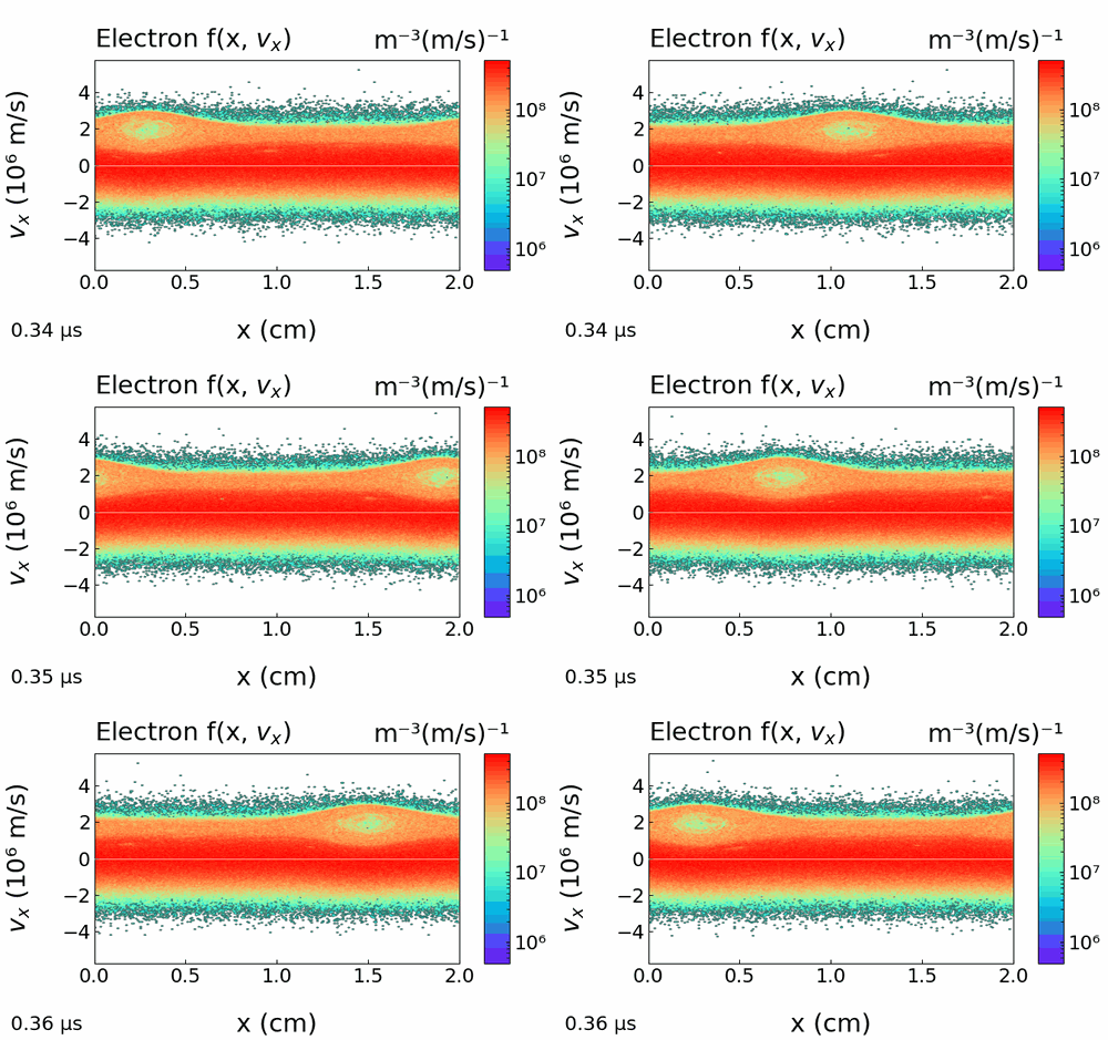
Figure 288: electron phase space (x, vₓ) during the growth of the instability.

The electron distribution is initialized as the combination of a stationary Maxwellian bulk and a faster electron beam of lower density (the beam may itself be a drifted Maxwellian). The instability is driven by a resonance between the beam particles and the Langmuir waves (plasma waves) of the bulk.

Key features to observe

1. Species Roles: Only a fraction of the total electron density (typically 1 to 10%) carries the drive energy. The bulk plasma provides the medium in which the waves propagate.
2. Phase Space Dynamics: Vortices (phase-space holes) form specifically within the beam population. The bulk plasma remains mostly centered at v=0, but it shows small-amplitude oscillations.
3. Saturation Mechanism: Saturation occurs by particle trapping. The beam electrons are trapped in the potential wells of the excited Langmuir waves. This “flattens” the distribution function and forms a plateau.
4. Energy Transfer: Kinetic energy of the beam is transferred into high-frequency electrostatic wave energy. Because the beam is dilute, the total heating of the system is smaller than in the Buneman case.

Dispersion relation and growth rate

The dense background (density $n_0$, plasma frequency $\omega_{pe}$) and the dilute cold beam (density $n_b$, velocity $v_b$, beam plasma frequency $\omega_{pb}^2 = (n_b/n_0)\,\omega_{pe}^2$) are treated as two cold electron fluids. The electrostatic response for perturbations $\propto \exp[i(kx-\omega t)]$ is then the sum of the two Langmuir terms. This gives the dispersion relation

The bulk term resonates at $\omega \simeq \omega_{pe}$ and the Doppler-shifted beam term at $\omega \simeq k v_b$. The coupling is strongest where the two coincide, that is, for the wavenumber $k v_b \simeq \omega_{pe}$. With $\omega = \omega_{pe} + \Delta$ and $|\Delta| \ll \omega_{pe}$ at $k v_b = \omega_{pe}$, the dispersion relation reduces to the cubic

Its two complex roots describe a wave that both propagates and grows. The maximum growth rate is

Because of the $1/3$ power, the growth remains appreciable even for a dilute beam: with $n_b/n_0 = 5\%$ here, $\gamma_{\max} \approx 0.25\,\omega_{pe}$. The unstable waves grow while they travel with the beam at the phase velocity $\omega/k \simeq v_b$. This is why the phase-space vortices develop inside the beam population and not in the bulk.

Conditions of the simulation

Collisionless neutral helium plasma Periodic boundary conditions, length d = 2 cm Initial total plasma density nₑ=nᵢ=10¹⁵ m⁻³ Electron beam energy $\varepsilon_b$ = 10 eV Fractional beam density 5% Electron bulk temperature Tₑ=5 eV Ion temperature Tᵢ=0.5 eV Number of grid points 200 Number of particles 1000000 Time step 5x10⁻¹¹ s

Pictures from the simulation

Electron phase space at t=0 The Maxwellian plasma and the electron beam (red line) are visible

Electron phase space as a function of time The phase space holes or vortices in the electron distribution are visible.

IX.A. Case 2 Beam Plasma Instability bounded

→ Go to Beam-Plasma Instability in a Thermionic Discharge

IX.A. Case 3 Buneman Instability

The Buneman instability is a fundamental current-driven plasma instability. It occurs when there is a large relative “drift” velocity between the electrons and the ions. (It should not be confused with the Farley-Buneman instability, which is a different, collisional, cross-field mode of the ionospheric E-region.)

It can be compared to a wake in a fluid: when the electrons move through a background of ions faster than a certain threshold, they cause a fast growth of electrostatic waves.

The Physical Trigger

For the instability to occur, the relative velocity between the electrons and the ions must be larger than the thermal velocity of the electrons. When this threshold is exceeded, the kinetic energy of the drifting electrons is converted into the potential energy of electric field oscillations.

How it Develops

The process can be summarized in three stages: 1. Perturbation: A small random fluctuation of the charge density occurs (this is natural in any plasma). 2. Resonance: The electrons “see” this fluctuation. Because they move very fast, they interact with the ion background in a way that creates a feedback loop. 3. Exponential Growth: The electric fields produced by the charge separation trap more electrons and create larger “bunches.” These bunches further increase the electric field, and the wave amplitude grows exponentially.

Key Mathematical Characteristics

The Buneman instability is a longitudinal electrostatic wave. In the cold-fluid description the electrons drift at velocity $v_d$ through the (mobile) ion background, and the electrostatic dispersion relation for perturbations $\propto \exp[i(kx-\omega t)]$ is

where $\omega_{pe}$ and $\omega_{pi} = \omega_{pe}\sqrt{m_e/m_i}$ are the electron and ion plasma frequencies. The Doppler-shifted electron term contains a slow, negative-energy beam mode. This mode resonates with the ion oscillation ($\omega \simeq 0$) when $k v_d \simeq \omega_{pe}$. Expanding around this resonance reduces the dispersion relation to the cubic

so the mode oscillates and grows at the same time, with

Its growth rate is one of the fastest in plasma physics, because it uses the collective motion of the entire electron population. Even with the $\left(m_e/m_i\right)^{1/3}$ scaling, the growth rate remains a large fraction of $\omega_{pe}$ (for helium, $\gamma_{\max} \approx 0.035\,\omega_{pe}$). The cold-fluid threshold requires the drift to be larger than the electron thermal speed, $v_d \gtrsim v_{th,e}$. This condition is largely satisfied here, because the imposed drift $v_d = 1.86\times10^{6}$ m/s (10 eV) is well above $v_{th,e}$ at $T_e = 5$ eV.

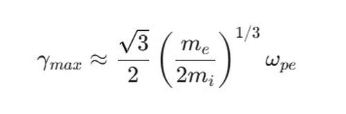
Figure 289: growth rate of the unstable branch of the dispersion relation (cold-fluid solution).

Effects and Consequences

When the Buneman instability “saturates” (reaches its limit), it causes several major changes in the plasma: Anomalous Resistivity: The plasma suddenly becomes much more resistant to the current than classical theory predicts. The “bunched” electrons collide effectively with the wave fluctuations. Plasma Heating: The energy of the drift motion is converted into heat, and the temperature of both electrons and ions increases rapidly. Turbulence: It often evolves into a state of plasma turbulence, which can disturb magnetic confinement in fusion devices (such as Tokamaks).

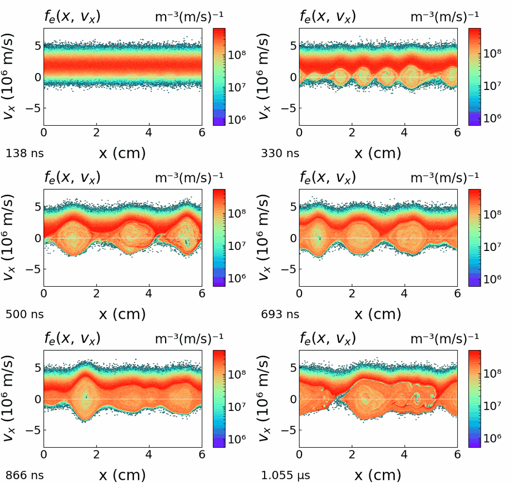
Figure 290: time evolution of the electron phase space (x, vₓ)

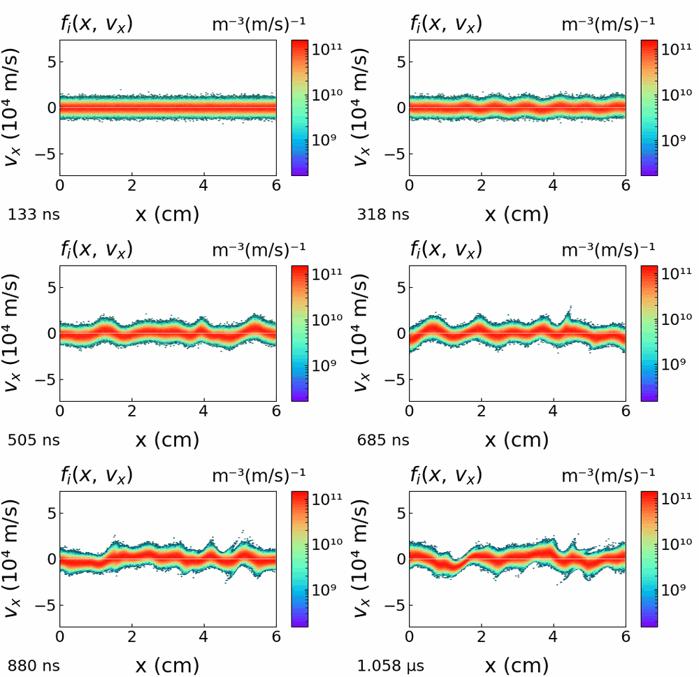
Figure 291: time evolution of the ion phase space (x, vₓ)

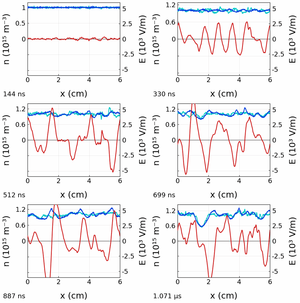
Figure 292: time evolution of the density and electric field profiles #### Conditions of the simulation Helium ion mass, pressure p=0 Pa Gap length d = 6 cm, periodic boundary conditions Plasma density 10¹⁵ m⁻³ Initial electron temperature 5 eV Superimposed electron drift 1.86x10⁶ m/s (10 eV) Initial ion temperature 0.5 eV Number of grid points 400 Number of particles 1000000 Time step 5x10⁻¹¹ s Click Run to see the development of the instability The instability forms in about 100 ns

IX.A. Case 4 Symmetric Two-Stream Instability

Principles

The two-stream instability is one of the most basic and most studied electrostatic instabilities in plasma physics. Its source is the free energy contained in the relative motion of the different plasma components. It is a classic example of the conversion of the kinetic energy of a directed particle beam into wave energy by collective plasma effects. The system is called symmetric when two identical particle beams, usually electron beams, move through a fixed neutralizing background of ions with equal and opposite velocities v₀ and -v₀. In this case the thermal spread of the beams is often neglected at first, in order to keep only the fluid mechanism. This configuration is called the cold symmetric two-stream instability.

Physics

The instability is driven by a feedback loop between the bunching of the particles and the space-charge electric field that this bunching produces. A small initial density perturbation in one of the streams changes the local electrostatic potential. This local electric field then modulates the velocities of the two streams, and the particles form stronger bunches. The beams move in opposite directions, so the Doppler-shifted frequencies of the plasma waves carried by each beam can be equal. The result is a resonant reinforcement with a fixed phase relation. The start and the growth of the instability are described by the longitudinal dielectric function. In the cold symmetric limit, the dispersion relation for electrostatic perturbations proportional to exp[i(kx-ωt)] becomes:

where $\omega_{pe}$ is the electron plasma frequency of a single beam, $k$ is the wavenumber and $\omega$ is the complex frequency. The two terms are the Doppler-shifted Langmuir responses of the $+v_0$ and $-v_0$ streams. When the denominators are removed, this relation becomes a bi-quadratic equation in $\omega^{2}$,

When this equation is solved, one branch $\omega^{2}$ becomes negative when $k v_0 < \sqrt{2}\,\omega_{pe}$. This gives a pair of purely imaginary frequencies $\omega = \pm i\gamma$. The root with $\gamma = \mathrm{Im}(\omega) > 0$ is the mode that grows exponentially, that is the unstable mode. The growth is fastest at $k v_0 = \frac{\sqrt{3}}{2}\,\omega_{pe}$, where it is equal to

This produces the rapid growth of the electric field. When the instability goes beyond the linear regime, the electric fields that grow exponentially act back strongly on the particle distributions. In this non-linear phase the particles are trapped in the electrostatic potential wells. This trapping forms the classic “phase-space vortices”, also called “holes.” The process finally saturates. The wave stops growing, the plasma is strongly heated, and the initial directed kinetic energy is thermalized.

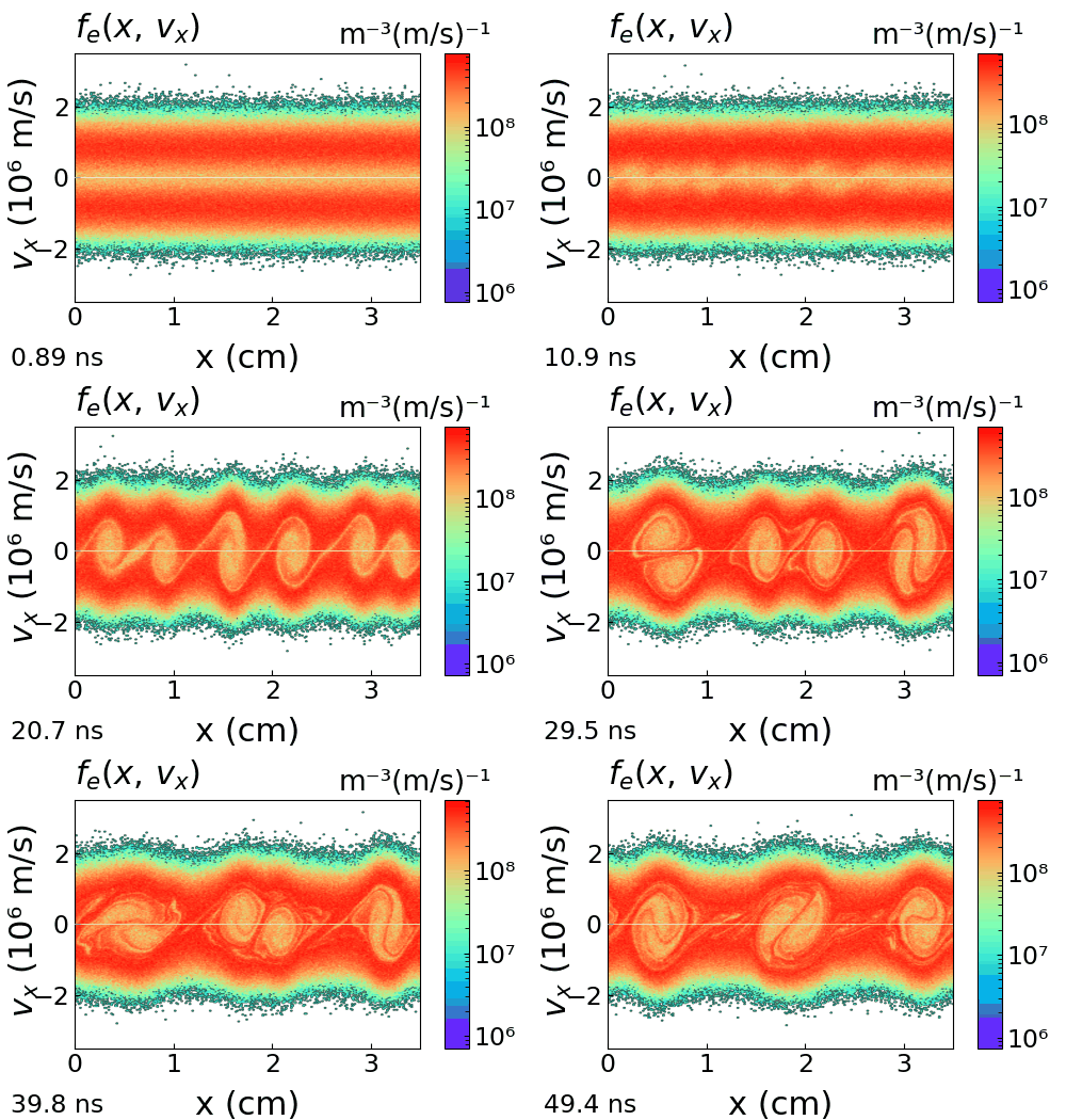
Figure 293: Time evolution of the electron phase space (x,vₓ). The conditions of the simulations are given below.

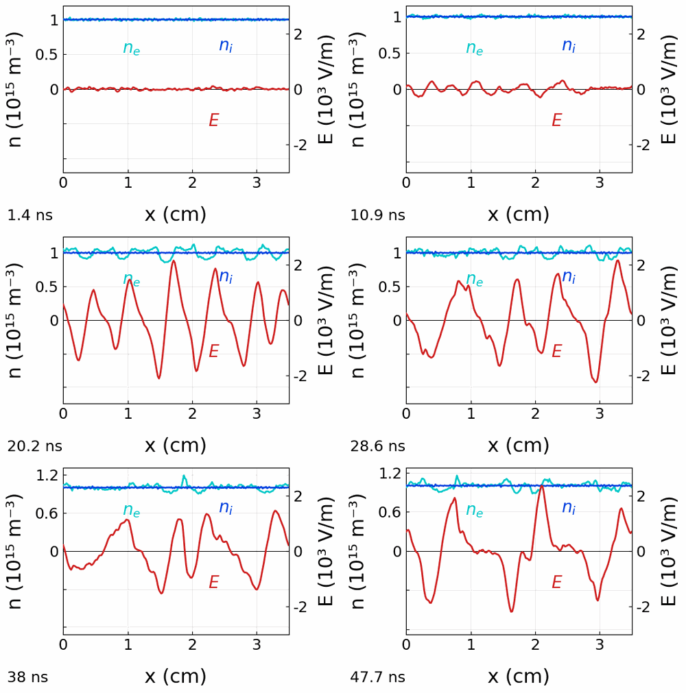
Figure 294: Time evolution of the spatial profiles of the electron and ion densities and of the electric field

Conditions of the simulations

Xenon ion mass (the ions have no role in this electron instability), pressure p=0 Pa Gap length d = 3.5 cm, periodic boundary conditions Plasma density 10¹⁵ m⁻³ Initial electron temperature 1 eV Superimposed electron drift stream 1 : 8.39x10⁵ m/s (2 eV) Superimposed electron drift stream 2 : -8.39x10⁵ m/s (2 eV) Initial ion temperature 1 eV Number of grid points 200 Number of particles 1000000 Time step 1x10⁻¹¹ s Click Run to see the development of the instability The instability develops in about 10 ns

IX.B Sheath Oscillations

The two examples of sheath oscillations presented in this section are both directly linked to the emission of electrons from the cathode:

Virtual Cathode Oscillations: This effect occurs in a vacuum diode (see the vacuum diode section) when the current of the injected electron beam is larger than the Child-Langmuir limit. The negative space charge that results produces a virtual cathode. This virtual cathode is dynamically unstable and oscillates in time.

Anode Glow Mode Oscillations: This occurs in thermionic discharges working in a low-pressure gas. At high enough current densities, the virtual cathode that forms near the emitter acts as a potential well. It traps the low-energy ions produced by charge-exchange collisions. The number of trapped ions increases and makes the virtual cathode unstable. The system then changes to a state in which a quasineutral plasma with zero field expands toward the anode. As a result, the ionization takes place only in a thin layer close to the anode. This configuration is unstable and produces low-frequency relaxation oscillations.

IX.B. Case 1 Virtual Cathode Oscillations

→ Go to Virtual Cathode Oscillations

IX.B. Case 2 Anode Glow Mode

→ Go to Anode Glow Mode (AGM) Self-Oscillations

IX.C Positive Column Striations

→ Go to Striations and Ionization Waves

IX.D ECDI - Hall Thrusters

→ Go to Hall Thruster — the E×B Electron Drift Instability

X Appendix

This chapter contains the material that the rest of the library assumes to be known. It is placed at the end because it is a reference rather than a progression, not because it is optional. A reader who is not sure what a Debye length actually screens, or what a cross section actually measures, will find the sheath and instability chapters more difficult than necessary.

Three sections, in increasing order of specificity.

Basic Concepts and Definitions collects the lengths, the frequencies, the velocities and the distributions of a plasma, and explains the physical meaning of each one. It ends by converting them into the numerical requirements of a particle simulation: the cell, the time step, the number of particles per cell. Four pages to read, nothing to run.

Single-Particle Motion is the only place in the library where the fields are imposed instead of being computed. This is what makes the orbits visible: the gyration, the cycloid and the E×B drift, an electric field along B compared with one across it, the gradient drift that separates the charges, the magnetic mirror and its loss cone, and finally the collisions that allow a particle to change field line. Eight interactive cases.

Collisions and Cross Sections opens the one physical ingredient that JC-PIC does not compute, the tabulated cross sections of the gas, and follows them to the algorithm that converts them into collisions. It begins with the classical description of a binary collision, in the centre of mass frame, and of the Coulomb collision. It then shows what the data actually contains, the mean free path and the collision frequency that follow from it, the null-collision method and the upper limit it imposes on the time step, the effect of a single collision, and the Maxwellian averages that connect all of this to fluid and global models. Seven interactive cases.

The last two sections run in modules of their own rather than in the PIC engine, and they answer in milliseconds instead of hours. They take from the engine everything that matters for the physics to be real: the Boris pusher, the null-collision Monte Carlo, and the cross-section files themselves.

X.A Basic Concepts and Definitions

A plasma is described by a small number of lengths, a small number of times and a small number of speeds. Almost every statement made anywhere in this library is a comparison between two of them. A sheath forms because the Debye length is small compared with the gap. A discharge is magnetised because the Larmor radius is small compared with the gap. It is collisional because the mean free path is small compared with the gap. It is expensive to simulate because the electron plasma period is short compared with the ion transit time. None of this is difficult. What is easy to lose is the physical meaning of each definition, and the orders of magnitude that make one of them dominate another.

These four pages collect these definitions and say what each one MEANS, and not only how it is computed. They are made to be read once and consulted again later, not to be run: there is nothing to launch.

Every number given here is computed for the same reference discharge, so the orders of magnitude remain attached to a concrete example. This discharge is argon at 100 mTorr and 300 K, an electron density of $10^{16}\ \mathrm{m}^{-3}$, an electron temperature of 3 eV, ions at the gas temperature, a magnetic field of 50 mT where one is needed, and a gap of 5 cm. This is a completely ordinary low-pressure capacitive discharge, and it is close to the conditions of several cases in the library. If any of these values is changed, the order of the scales changes as well, and this is exactly the important point.

The last page converts the physical scales into the numerical ones: the cell, the step, the number of particles. In a particle simulation these are not two separate subjects.

X.A. Case 1 Lengths: Debye shielding and the others

A plasma is not characterised by one length but by four. Almost every statement in this library is a comparison between two of them. They are collected here for the reference discharge described in the section introduction, so that the orders of magnitude are attached to a concrete example.

The Debye length Consider a test charge placed in a plasma. The electrons are mobile: they move towards the charge if it is positive and away from it if it is negative. The charge that they redistribute cancels the field of the test charge. The electron density is written as a Boltzmann factor of the potential and inserted into Poisson’s equation. For a small potential, the result is an exponential decay instead of the Coulomb tail:

with the temperature in volts. This is the meaning of “an electron temperature of 3 eV”. The Debye length is therefore the distance beyond which a charge is not seen. Two consequences follow immediately. On scales much larger than the Debye length a plasma is neutral, not because the charges are paired but because any imbalance is screened. On scales comparable with the Debye length, neutrality fails. For this reason every sheath in this library is a few Debye lengths thick. In the reference discharge, λ_D = 0.129 mm.

The screening argument is valid only if there are many electrons inside the screening volume; otherwise there are no electrons to do the screening. This condition is the plasma parameter,

which is about 21 thousand here. When it is large, the plasma is collective, and the binary Coulomb collisions treated in the Collisions section are a small correction. When it approaches unity, the plasma is strongly coupled and none of these results apply.

The Larmor radius In a magnetic field a particle rotates on a circle of radius

and the whole Single-Particle Motion section is based on this quantity. The electron and ion radii are very different, and not in the direction that the mass ratio suggests. The ion is heavier, but it is also much slower. At equal TEMPERATURE the ratio of the radii is the square root of the mass ratio. Here, with 50 mT, $r_{L,e}$ = 0.117 mm for a 3 eV electron and $r_{L,i}$ = 2.949 mm for an ion at the gas temperature.

The mean free path The distance between two collisions,

depends on the gas density, and therefore on the pressure, and on the energy through the cross section. In argon this energy dependence is strong because of the Ramsauer minimum. At 100 mTorr and 3 eV it is λ = 7.580 mm. Compared with the 5 cm gap, this gives 7 collisions across the discharge. The discharge is collisional, but not by a large margin. A slower electron in the Ramsauer window would cross the discharge without any collision.

Figure

Figure 295: on the left, the potential of a test charge with and without the plasma around it. The screened potential is reduced by a factor e at one Debye length and by a factor 150 at five Debye lengths. On the right, the four lengths of the reference discharge on a logarithmic axis, with the size of the gap for comparison.

What to remember

The ordering of these lengths IS the physics of a case. A sheath exists because the Debye length is small compared with the gap. A discharge is magnetised because the Larmor radius is small compared with the gap. It is collisional because the mean free path is small compared with the gap. If the pressure, the density or the field is changed, the ordering changes, and the result changes with it.

X.A. Case 2 Frequencies: plasma, cyclotron, collision

This is the same exercise, now in time. A plasma has its own characteristic frequencies, and they cover five decades. A simulation must resolve the fastest one and must run long enough to see the slowest one. This is what makes kinetic simulation expensive.

The plasma frequency All the electrons of a slab are displaced by a distance x, and the ions stay where they are. The uncompensated charge creates a uniform field that pulls the electrons back. This field is proportional to the displacement, so the electrons oscillate as a harmonic oscillator:

This is the fastest spontaneous motion of a plasma, and it depends only on the density. It does not depend on the temperature, on the field or on the gas. It gives the speed at which a plasma restores its own neutrality, and it is the frequency of the Langmuir waves of the Basic Plasma Physics chapter. The ions oscillate in the same way with their own mass,

which for argon makes them 271 times slower. This single ratio produces the two time scales of every discharge in this library. Here $5.641\times10^{9}$ rad/s, that is 898 MHz, and $2.080\times10^{7}$ rad/s, that is 3.31 MHz.

The cyclotron frequency The rate at which a particle rotates in a magnetic field,

depends only on the field and on the mass. It does not depend on the speed, so the gyration gives a fixed frequency and not only a circle. At 50 mT the electron rotates at 1.40 GHz and the argon ion at 19 kHz.

The collision frequency, and the two ratios that matter An electron collides with the neutral gas at

which is $1.355\times10^{8}$ s⁻¹ here. Two comparisons determine the behaviour of the discharge. The first one is with the cyclotron frequency,

the Hall parameter is 64.9 here, so the mobility across the field is reduced by a factor 4211. The magnetic field therefore does confine the particles. The second comparison is with the driving frequency of an RF discharge: there are 1.6 collisions per radian at 13.56 MHz. This number determines whether the electrons follow the field or drift through it.

And the Coulomb frequency Electrons also deflect each other. This rate is not a cross section multiplied by a density in the usual sense, and the derivation is given in the Collisions and Cross Sections section. Its order of magnitude follows from

with the density in cm⁻³ and the temperature in eV. Here ln Λ = 13.1 and ν_ei = $7.36\times10^{4}$ s⁻¹, which is 1842 times slower than the collisions with the neutral gas. This is the usual situation in a low-temperature discharge with an ionisation degree of a fraction of a percent. For this reason JC-PIC keeps the Coulomb collisions switched off by default.

Figure

Figure 296: the characteristic frequencies of the reference discharge on a logarithmic axis, with the RF driving frequency for comparison. A simulation must advance faster than the leftmost one and must run longer than the rightmost one.

What to remember

This hierarchy is the reason why a PIC code is written in this way. The time step is fixed by the electron plasma frequency, at the fast end. The physics that is usually of interest, the ion dynamics and the steady state, is at the slow end, thousands of times further away. Every part of the code that looks like an optimisation, including ion subcycling, is an attempt to avoid the cost of the full ratio.

X.A. Case 3 Velocities, temperatures and distributions

Temperature is the point where the language of fluids and the language of particles separate. Most of the confusion in reading kinetic results starts here.

Temperature in volts, and the three thermal speeds A temperature is an energy, and plasma physics gives it in electron volts: 1 eV is 11605 K. It is a property of a DISTRIBUTION, not of a particle. A single electron has an energy, never a temperature. A distribution has a temperature only if it is Maxwellian, and in a discharge it is usually not Maxwellian. Three different speeds are all called thermal. They differ by tens of percent, which is enough to lose a factor in an estimate:

At 3 eV, the mean speed is $1.16\times10^{6}$ m/s and an electron of exactly 3 eV moves at $1.03\times10^{6}$ m/s.

The speeds that are not thermal Two velocities are set by the electron temperature but belong to the IONS. They control every boundary in this library. The Bohm speed,

is $2.68\times10^{3}$ m/s here, that is, 8 times the thermal speed of the ions themselves. Ions arrive at a wall at supersonic speed because the electrons accelerate them, not their own temperature. The ion acoustic speed is the same expression with the ion temperature added. It is the speed of the waves of the Ion Acoustic Waves section.

The distribution, and how to read it The quantity that a kinetic code actually produces is the distribution of electron energies. It is almost always plotted as the electron energy PROBABILITY function and not as the distribution function,

for one reason: on a logarithmic vertical axis a Maxwellian is then a STRAIGHT LINE, with a slope equal to minus one over the temperature. Any departure from a straight line is a departure from a Maxwellian. It is visible immediately, and these departures are the purpose of a kinetic simulation. A depleted high-energy tail is the rule and not the exception, because the inelastic thresholds remove electrons from the tail faster than the elastic collisions can replace them. A Druyvesteyn distribution, whose logarithm decreases as the SQUARE of the energy instead of linearly, is the classic result when only elastic collisions and a constant field are present. This is important well beyond the plot. Ionization is produced by the electrons above 15.8 eV in argon, that is, by electrons five temperatures out in the tail. There the population is exponentially small, and a Maxwellian assumption can be wrong by an order of magnitude. This is the difference between the rate coefficients of the Collisions section, which assume a Maxwellian, and those computed by the swarm solver.

Figure

Figure 297: Maxwellian energy probability functions at three temperatures (straight lines, slope −1/Te), with a Druyvesteyn distribution of the same mean energy for comparison. The two agree at low energy and differ by orders of magnitude in the tail that produces the ionization.

What to remember

Give a temperature only for a distribution that you have examined. When reading a kinetic result, first plot the EEPF on a semi-logarithmic axis. This takes one second, and it shows whether any of the fluid formulas apply at all.

X.A. Case 4 From the physical scales to the numerical ones

The lengths and times of the three previous pages are not only descriptive: they are the specification of the simulation. Every constraint that a JC-PIC input file has to satisfy is one of them. The cost of a run is the ratio between the smallest scale that must be resolved and the largest scale that must be reached.

The cell must resolve the Debye length The explicit PIC scheme is numerically unstable when the cell is much larger than the Debye length. The finite-grid instability heats the plasma artificially until the Debye length has increased to the cell size. This looks like physics, but it is not. Therefore

With λ_D = 0.129 mm and a 5 cm gap, this gives at least 389 cells. Four times more cells are needed if the density is sixteen times higher, because the Debye length decreases as one over the square root of the density.

The step must resolve the plasma frequency The same scheme is unstable unless the electrons are advanced fast enough to follow their own oscillation:

Here this gives 35.5 ps. Two further upper limits apply at the same time. The first is the Courant condition: a particle must not cross a cell in one step,

The second is the collision limit of the Monte Carlo part, which is the subject of the Collisions and Cross Sections section:

in which ν_max is not the collision frequency at the mean energy but the upper bound of the null-collision method, $1.04\times10^{9}$ s⁻¹ for argon at 100 mTorr. This limit is 192 ps, five times less strict than the 35 ps required by the plasma frequency. So here the density decides. This is not always the case. The collision limit does not depend on the density at all, while the plasma-frequency limit decreases as one over the square root of the density. So below about $3.4\times10^{14}$ m⁻³ at this pressure the collisions become the stricter limit. Increasing the pressure moves this crossing to a higher density.

The particles are a statistical sample A PIC particle is not an electron. It is a macroparticle that represents a large number of electrons. Every quantity computed from the macroparticles carries a sampling noise, which decreases only as the square root of the number per cell,

So a hundred particles per cell gives ten percent noise on the density, and more on any quantity computed from the tail of the distribution. Doubling the accuracy costs four times the run time. This is the reason why a rate coefficient converges much more slowly than a density. It is also the reason why it is useful to watch the convergence of the free-flight histogram of the Collisions section.

And the ratio that sets the bill The step is set by the electrons and the duration by the ions:

which is 271 for argon. Reaching a steady state of the ion dynamics therefore costs of the order of a hundred thousand steps before anything has reached equilibrium, whatever the machine. Ion subcycling advances the ions once every few electron steps. It is the method used by JC-PIC to avoid paying this ratio twice.

Figure

Figure 298: the largest usable cell and the largest usable step as a function of the electron density, with the reference discharge marked. The dashed line is the null-collision limit for argon at 100 mTorr, which does not depend on the density at all. To the right of the crossing the plasma frequency decides; to the left the collisions decide.

What to remember

Before running anything, compute the Debye length and the plasma frequency for the expected density. They give the cell and the step directly, and therefore the cost of the run, before a single line of the input file has been written. Most simulations that “behave strangely” are simulations in which one of these two inequalities was violated.

X.B Single-Particle Motion

Before a plasma can be treated as a medium, the motion of a single charged particle in given fields must be clear. This section presents that basis. It is the only section of the library in which the fields are imposed and not computed. This is not a limitation but a choice: a trajectory can be read only when the field that produced it is known exactly.

The cases run in a separate module and not in the PIC engine. The reason is simple. Following a cycloid in a self-consistent simulation would need hours of computation, while the integration of the equation of motion gives the same result in milliseconds. The module takes from the engine everything that is needed for the physics to be correct. It uses the Boris scheme, so that the orbits are the same as those the engine would produce. It also uses the cross sections of ELECSCAT.DAT and IONSCAT.DAT, so that the cases with collisions show argon with its Ramsauer minimum and not a constant collision frequency.

Eight configurations are proposed, in the order in which they build on one another. A uniform magnetic field alone gives the gyration. It also gives the two quantities used as references in all the later cases, the Larmor radius and the cyclotron period. An electric field added across the magnetic field gives the cycloid and the E×B drift. This drift carries electrons and ions at the same velocity and in the same direction, whatever their mass and their charge. The same electric field placed along B gives free acceleration and does not change the gyration. The difference between these two cases is the basic idea of magnetic confinement. An oblique field reproduces the geometry of the magnetised sheath treated in the Basic Plasma Physics chapter. A magnetic field that varies in space gives the gradient drift. Unlike the E×B drift, this drift sends the two signs of charge in opposite directions, so it separates the charges. A magnetic field that converges gives the magnetic mirror, its loss cone and the conservation of the magnetic moment. Collisions, finally, are what allow a particle to change field line, and therefore what allows a magnetised plasma to reach a wall that lies across the field.

Each case opens with its own settings, which are locked, so that the screen shows exactly what the description says. One button unlocks them. The last case, Free exploration, starts unlocked with every control available. Any of the configurations can be reached from the list at the top of its panel.

The panel beside the plot prints the numbers that each figure is meant to show. It also indicates when the picture cannot have its usual meaning. One case is when a quantity does not vary at all. Another case is when the field varies too fast over one orbit for a guiding-centre drift to be defined. A third case is when the trajectory is too elongated for the two scales to be kept equal. These warnings are part of the teaching. The formulas of this section are approximations, and the module indicates where they are no longer valid.

X.B. Case 1 Gyration in a uniform magnetic field

This is the simplest motion that a magnetic field can produce, and all the other cases are based on it. A magnetic field does no work, because the force is always perpendicular to the velocity. The speed therefore never changes and the particle moves on a circle [142].

Field configuration

• Magnetic field: 50 mT, perpendicular to the plane of the figure
• Electric field: none
• Particle: an electron of 4 eV, injected at 90 degrees to the field
• Collisions: none
• Window: 6 cyclotron periods

The physics

The radius increases with the momentum perpendicular to the field, and it decreases when the field increases,

while the period does not depend on the speed,

What you see

The orbit closes on itself. After six turns the particle is back at its starting point. This result is not easy to obtain numerically, and this is the reason why the engine uses the Boris scheme [143]. The dashed curve is the same motion integrated with an explicit Euler scheme, with the same time step. This curve is a spiral that moves outward, because the Euler scheme adds energy at every step. The Boris rotation is exact, so the speed is conserved to machine precision. The circle remains a circle for any duration of the calculation.

Figure

Figure 299: An electron of 4 eV in 50 mT, during six cyclotron periods. The Boris orbit closes. The explicit Euler orbit gains energy and opens.

Things to try

Change B: the radius varies as 1/B, and the period varies in the same way. The number of turns that is drawn stays the same, because the window is counted in cyclotron periods. Change the energy instead: the radius increases and the period does not change.

X.B. Case 2 An electric field across B: the cycloid and the E×B drift

When an electric field perpendicular to the magnetic field is added, the circle becomes a cycloid [142-143]. The particle is no longer fixed at one place. Its centre moves, and it moves across both fields.

Field configuration

• Magnetic field: 50 mT, perpendicular to the plane of the figure
• Electric field: 50 V/cm, perpendicular to the magnetic field
• Particle: an electron of 4 eV, launched at 90 degrees to the field, together with a helium ion of the same perpendicular speed
• Collisions: none
• Window: 6 cyclotron periods

The physics

The drift velocity is

and its magnitude is

What you see

The electron and the ion turn in opposite directions, because their charges have opposite signs. However, they drift in the SAME direction and at the SAME speed. The drift velocity does not depend on the mass, on the charge or on the energy. For this reason an E×B drift moves the whole plasma together instead of separating it, and for this reason it does not produce a current by itself. Here the lengths are measured in the Larmor radius of each particle, and both particles start with the same perpendicular speed. This is the only way to draw the two orbits on the same axes. At the same speed, as here, the ion radius is larger than the electron radius by the mass ratio itself, 7300 in helium. The ion period is larger by the same factor. At the same energy the ion radius would still be larger, by the square root of this ratio, 85.

Figure

Figure 300: An electron and a helium ion with the same perpendicular speed, in 50 mT with 50 V/cm perpendicular to the field. The gyrations are opposite, the drifts are identical.

Things to try

If E is increased, the arches of the cycloid open, until the orbit no longer makes loops. If B is decreased instead, the drift increases as 1/B, and the radius increases in the same way.

X.B. Case 3 An electric field along B: free acceleration

This case uses the same two fields as the previous case, but they are now parallel instead of perpendicular. The result is completely different. The difference between the two cases is the whole idea of magnetic confinement [142-143].

Field configuration

• Magnetic field: 50 mT, perpendicular to the plane of the figure
• Electric field: 5 V/cm, along the magnetic field
• Particle: an electron of 4 eV, launched at 85 degrees to the field
• Collisions: none
• Window: 8 cyclotron periods

The physics

Along the field the magnetic force is zero, and the motion is a free acceleration,

What you see

The gyration across the field is not changed. Its radius and its period are exactly those of the first case. Along the field the particle only accelerates, and the helix becomes longer at each turn. A magnetic field holds a particle on a field line, but it does not act at all on the motion along that line. A magnetic field confines a particle in two directions out of three only.

Figure

Figure 301: An electron in 50 mT with 5 V/cm along the field. The gyration is unchanged, and the pitch of the helix increases.

Things to try

Set the pitch angle to 90 degrees. The particle then starts with no velocity along B, and the field accelerates it from rest. Change the sign of the charge by showing the ion. The ion is accelerated in the other direction, and this is exactly what an E×B drift does not do.

X.B. Case 4 A field oblique to the wall: the Chodura geometry

This case is the geometry of a magnetised sheath, reduced to a single particle [142-143]. The wall is on the left and its normal is x. The magnetic field lies in the plane of the figure, at an angle to the wall. The electric field points along the normal, as it does in front of any surface in contact with a plasma. This is the configuration simulated in the oblique-sheath section of the Basic Plasma Physics chapter. The convention for the angle is the same as the one used by the engine.

Field configuration

• Magnetic field: 50 mT, at an angle of 30 degrees to the wall
• Electric field: 10 V/cm, along the normal to the wall
• Particle: an electron of 4 eV, launched at 90 degrees to the field
• Collisions: none
• Window: 10 cyclotron periods

The physics

The electric field is separated into two parts. The part along B accelerates the particle freely. The part across B only produces a drift:

What you see

The particle moves towards the wall, but it moves ALONG the field line, and not along the electric field. Only the component of E along B accelerates it. The perpendicular component only displaces its centre sideways. When the angle to the wall is smaller, this parallel component is smaller and the particle needs more time to arrive. For this reason a grazing field produces a much thicker layer in front of the wall than a field along the normal. For the same reason Chodura’s condition is written along the field and not along the normal [13].

Figure

Figure 302: An electron in a field at 30 degrees to the wall, with 10 V/cm along the normal. The motion follows the field line and not the electric field.

Things to try

Set the angle to 90 degrees. The field is then along the normal and the case reproduces the previous one exactly. The engine uses this same equality as a check. Set the angle to 5 degrees instead: the motion towards the wall almost stops.

X.B. Case 5 A field that varies in space: the gradient drift

The magnetic field is still perpendicular to the plane of the figure, but its strength now increases across the plane. It is 4 mT on the left of the box and 20 mT at the peak, over a scale of 4 mm. The electron starts on the side of that profile, where the gradient is largest. Its orbit is no longer a closed circle. It is wider where the field is weak and narrower where the field is strong. For this reason the orbit does not close, and its centre moves [142-143].

Field configuration

• Magnetic field: perpendicular to the plane, 4 mT at the ends and 20 mT at the peak, over a gradient scale of 4 mm
• Start position: 22 mm, on the side of the profile
• Electric field: none
• Particle: an electron of 4 eV, launched at 90 degrees to the field
• Collisions: none
• Window: 25 cyclotron periods

The physics

The centre of the orbit drifts perpendicular to the field and perpendicular to its gradient,

and the drift is defined only if the field varies over a length much larger than the orbit,

What you see

The field increases towards the right, so the drift is directed downwards along y. It is perpendicular to B, which comes out of the page, and perpendicular to the gradient, which points to the right. Each turn moves the orbit by about one fifth of a Larmor radius, and the twenty-five loops of the figure go down one after the other. The thick line is the guiding centre, that is the position of the orbit with the gyration removed. This last curve is not only a convenience. Here the field varies over seventeen Larmor radii, and this separation of scales is what gives a meaning to the drift. Because of it, each turn moves the orbit by only a small fraction of a radius. If the separation of scales is made larger, the loops overlap and form a solid band in which nothing can be read. Only the guiding centre still shows the motion. The second figure shows the same result in another way. Against time the guiding centre is a straight line, and the drift velocity can be measured from its slope. Two properties of this drift must be remembered. It does not depend on the mass, because at a given energy the numerator is equal to twice the perpendicular energy. However, it depends on the sign of the charge, so a positive particle drifts in the opposite direction. A plasma placed in a gradient of B therefore separates its charges. This is the origin of the E×B instabilities studied later in this library. The module can show this. The switch “positive charge of electron mass” adds a particle that drifts exactly like a real ion, with an orbit small enough to be drawn on the same axes.

Figure

Figure 303: An electron of 4 eV in a field increasing from 4 to 20 mT over 4 mm, during twenty-five cyclotron periods. The loops move downwards. The thick line is the guiding centre.

Figure 304: The same trajectory shown against time. The guiding centre is a straight line, and its slope is the drift velocity: 2 mm in 55 ns, that is $3.6\times10^{4}$ m/s. The gyration is the small oscillation around this line. This view is obtained in the module with the plot selector set to t – y.

Things to try

Move the start position to the flat part of the profile. The drift stops, because there is no gradient there. Reduce the gradient scale until it becomes close to the Larmor radius. The guiding centre is then no longer a straight line. The drift is no longer defined, and the panel indicates this. The panel prints the ratio of the field scale to the Larmor radius, and this ratio is the number that decides.

X.B. Case 6 A field that converges: the magnetic mirror

The field is now along the axis. It is weak in the middle and strong at both ends: 18 mT at the centre of the trap and 60 mT at each end. A particle launched in the middle is turned back before it reaches an end, if a large enough part of its velocity is across the field. This is the oldest idea of magnetic confinement, and the only one that needs no electric field at all [142-143].

Field configuration

• Magnetic field: along the axis, 18 mT in the middle and 60 mT at both ends
• Electric field: none
• Particle: an electron of 4 eV, launched at 45 degrees to the field
• Collisions: none
• Window: 60 cyclotron periods

The physics

The magnetic moment is conserved as the particle moves along the field,

The energy is conserved too, so the particle turns back where the field reaches

and every particle launched inside the loss cone escapes:

What you see

Panel (a) shows the motion itself: a helix that turns around a field line. The helix becomes narrower where the field lines converge and wider again in the middle. The dashed lines are the field lines, drawn with the exact relation that defines a flux tube, r(x) = r_0 sqrt(B_0/B(x)). The thick line is the guiding centre. It moves back and forth along the axis while the particle turns around it. The transverse scale is exaggerated: about thirty millimetres of axis against a quarter of a millimetre of radius. Panel (b) shows the same motion as a function of time, together with a second particle that differs only by its pitch angle. At 45 degrees the particle is reflected. At 20 degrees, inside the loss cone, it crosses the trap and is lost at the wall. Panel (c) gives the reason. When the particle moves into the stronger field, energy passes from the motion along the field to the motion across the field. The two curves are exactly the field profile, scaled. The black dashed line is B(x)/B_0 multiplied by the square of the sine of the launch angle, and the measured perpendicular fraction lies on it. This is the conservation of the magnetic moment, seen directly and not only stated. The particle turns back at the point where the perpendicular part carries all the energy and the parallel part is equal to zero. Panel (d) shows why one particle is trapped and the other is not. For each launch angle there is a field value at which the particle would turn back, and the only question is whether the trap reaches this value. At 45 degrees this field is 36 mT, well below the 60 mT of the ends. The shaded band is the part of the axis that the particle visits. At 20 degrees a field of 154 mT would be needed, and the trap never gives it. There is no force along the field in the usual sense. The particle is turned back by the small radial component that a converging field must have, acting on the gyration. This is also why the effect depends on the angle and not on the energy.

Figure

Figure 305: An electron of 4 eV in a mirror, 18 mT in the middle and 60 mT at both ends, launched at 45 degrees. The loss-cone angle is 33 degrees.

Things to try

Decrease the pitch angle below the loss-cone angle, which is printed in the panel: the particle then crosses the trap and stops at the wall. Increase the ratio of the end field to the middle field, and the loss cone becomes narrower. The 3D button opens the trajectory in space in a separate window, which can be turned with the mouse.

X.B. Case 7 Collisions across B: how a particle crosses field lines

A magnetic field alone keeps a particle on the same field line for ever. Collisions allow the particle to change field line. They are therefore what allows a magnetised plasma to reach a wall placed across the field [142-143]. Each red dot on the figure is one collision. The collisions are computed with the same cross sections as those used by the engine. The argon used here has its Ramsauer minimum, so the collisions become rare below one electron volt.

Field configuration

• Magnetic field: 50 mT, perpendicular to the plane of the figure
• Electric field: 8 V/cm, across the magnetic field
• Particle: an electron of 4 eV, launched at 90 degrees to the field
• Gas: Ar at 300 mTorr, 300 K, with the cross sections of ELECSCAT.DAT
• Window: 200 cyclotron periods

The physics

Between two collisions the guiding centre does not move. At each collision it moves by about one Larmor radius. The mobility across the field follows,

What you see

The guiding centre performs a random walk across the field while it drifts along the field. One number determines how easily the particle crosses the field: the ratio of the cyclotron frequency to the collision frequency. The panel prints this ratio and the mobility ratio that follows from it. When this ratio is large, the particle stays on its field line and moves very little across it. When the ratio approaches one, the field has almost no effect.

Figure

Figure 306: An electron in argon at 300 mTorr, in 50 mT with 8 V/cm across the field. Red dots mark the collisions. The thick line is the guiding centre.

Things to try

Change the pressure over two decades and observe how the random walk changes. The mobility ratio in the panel is the theoretical value for comparison. The trajectory is one realisation, and New draw gives another one.

X.B. Case 8 Free exploration

This is the same module, with nothing locked. Every case of this section can be reached from the Case list at the top of the panel, and every control is active. Use this case to answer the questions raised by the other cases [142-143].

Field configuration

• Magnetic field: 50 mT, perpendicular to the plane of the figure
• Electric field: 50 V/cm, across the magnetic field
• Particle: an electron of 4 eV, launched at 90 degrees to the field, together with a helium ion of the same perpendicular speed
• Collisions: none
• Window: 6 cyclotron periods

What you see

The panel under the controls is not a decoration. It prints the numbers that the figure is meant to show. These are the cyclotron frequencies and periods, the Larmor radii and their ratio, and the drift velocity. It also prints the collision frequency and the cross-field mobility that follows from it, the length over which the field varies, measured in Larmor radii, and the width of the loss cone. It also indicates when the picture on the screen cannot have its usual meaning. One case is when a quantity does not vary at all and is drawn as a flat line instead of rounding noise. Another case is when the trajectory is too elongated for the scales to be kept equal. A third case is when the field varies too fast for a guiding-centre drift to be defined. Play animates the trajectory, and the recorder writes it as a GIF, in the same format as every other movie in this library.

Figure

Figure 307: The starting point, an electron and an ion in crossed fields, with every control available.

Things to try

The mouse actions are useful to know. Drag inside the plot to move the origin. Drag over the tick numbers of one axis to move this axis alone. Use the wheel to change the scale of the axis under the pointer. The right button moves the plot inside its window. A border changes its size, and a double-click inside restores the automatic framing.

X.C Collisions and Cross Sections

The cross sections are the only physical ingredient that JC-PIC does not compute. The fields are obtained from Poisson’s equation, the trajectories from the equation of motion, and the sheaths and the waves from the two together. But the probability that an electron collides with an atom, and the effect of that collision, are measured data read from a file. All data in that file are taken from LXCat, an open-access database that can be found at www.lxcat.net [37]. These data are shown in a few dozen curves in DATA/ELECSCAT.DAT and DATA/IONSCAT.DAT, and this section opens that file. Note that additional data for gases not included in these files can also be found on the LXCat site [37] [144].

Before looking at the data, it is useful to recall what a cross section measures, and what a collision does. The three sub-sections that follow are classical kinetic theory, textbook material [5]. They are given here because the rest of the section assumes them.

The two-body collision

Two particles of masses m and M approach each other. In the laboratory frame the problem has six unknown velocity components after the collision. In the frame of the centre of mass it has only one unknown: the angle through which the pair is deflected. That frame moves at

and it is not affected by the collision, because momentum is conserved. The remaining quantity is the relative velocity. For an elastic collision it only changes direction and keeps its magnitude:

The energy available for any inelastic process is the kinetic energy in that frame, and the reduced mass appears in it:

This is not a formality. It is the reason why the engine computes the energy of an ion-neutral collision as one quarter of M g squared, and not from the laboratory speed of the ion. It is also the reason why the threshold of an inelastic process is a threshold in the centre-of-mass energy.

The fraction of energy given up by the projectile follows from the same two conservation laws alone, without any knowledge of the force between the particles:

Everything about a discharge follows from the two limits of this single expression. For an electron on an atom, the mass ratio makes this fraction 2m/M, which is $2.72\times10^{-5}$ in argon. An electron needs about 37 thousand elastic collisions to lose its energy. For an ion in its own parent gas the masses are equal and the factor is one half. An ion is stopped in a few collisions. This single contrast is the reason why a low-pressure discharge keeps the electrons at tens of thousands of kelvin while the gas and the ions remain at room temperature. It is the assumption behind every case in this library.

Figure 308: the same elastic collision, shown twice. On the left, in the laboratory frame: the incident particle of mass m arrives with an impact parameter $b$ onto a target M at rest. The impact parameter is the perpendicular distance by which the particle would miss the target if it moved in a straight line. The target is taken at rest because a gas atom is nearly still compared with the fast projectile. The projectile leaves at an angle $\theta$, and the target recoils at $\varphi$. On the right, the same event seen from the centre of mass, where the only change is a rotation by $\chi$. Every angle and every length is computed from the conservation laws for a mass ratio $m/M = 1/4$ and $\chi = 60^\circ$. Only the recoil arrow is drawn three times too long, because at this mass ratio it would otherwise be barely visible. For an electron on an argon atom it would be forty thousand times too short to be drawn at all.

Cross sections: differential, total, momentum transfer

The force between the two particles enters only through the probability of each deflection angle. The differential cross section is defined so that the number of collisions per unit time sending the pair into a solid angle dOmega is N g times it. Integration over all angles gives the total cross section. This is the quantity needed by the null-collision method [145], because that method only asks WHETHER a collision happened:

Transport, however, does not depend on the total cross section. A collision that deflects a particle by one degree removes almost none of its momentum along the original direction. A hundred such collisions have less effect than one backscatter. The quantity that controls mobility, diffusion and the drift velocity is therefore the MOMENTUM-TRANSFER cross section,

This is the quantity that the LXCat tables give for the elastic channel. It is also the reason why two very different angular distributions with the same $\sigma_m$ produce the same measured mobility. JC-PIC uses this invariance explicitly. When the anisotropic option is switched on [82], the elastic cross section is increased to $\sigma_m$ divided by the mean of $(1-\cos\chi)$ over the angles actually drawn. The product is then exactly $\sigma_m$. The number of collisions changes, the angular distribution changes, and the transport does not change.

Figure 309: on the left, four exact Coulomb orbits. The closer the particle passes, the more strongly it is deflected. The relation is $\tan(\chi/2) = b_{90}/b$, where $b_{90}$ is the impact parameter that produces a right-angle deflection. On the right, the definition of the differential cross section. The particles that come in through the ring between $b$ and $b+db$ are exactly those that go out through the cone between $\chi$ and $\chi+d\chi$. The definition simply states that these two groups are the same particles.

Coulomb collisions

Between two charged particles the interaction has no finite range. The deflection follows the Rutherford cross section,

whose integral over all angles DIVERGES. The total cross section is infinite, because a distant particle is always deflected a little. Two consequences follow. They are the reason why this section treats Coulomb collisions separately from all the others.

The first consequence is that the divergence has to be cut off. The physical cut-off is the Debye length of the appendix: beyond it the charge is screened and there is nothing left to deflect. When the cut-off is carried through the momentum-transfer integral, a logarithm remains. It is the only trace of the two limits:

In the reference discharge of the appendix (argon, $10^{16}\ \mathrm{m}^{-3}$, 3 eV), the impact parameter for a right-angle deflection is about 0.25 nm, against a Debye length of 0.129 mm. The logarithm of the ratio is 13.1. It is always of order ten. This is why its exact value is rarely a concern.

The second consequence is more important. The integral is dominated by its lower limit. Therefore a charged particle is deflected through a right angle not by one encounter but by the accumulation of many very small ones. Their number is about eight times the Coulomb logarithm. A Coulomb collision is therefore not an EVENT but a diffusion in velocity space. The null-collision method of this section, which asks whether a discrete collision happened during the step, does not describe it. Its rate is, for reference [146],

with the density in $\mathrm{cm}^{-3}$ and the temperature in eV. This gives $7.36\times10^{4}\ \mathrm{s}^{-1}$ here, which is 1842 times slower than the collisions with the neutral gas at 100 mTorr. This ratio is the usual situation in a low-temperature discharge, ionised at a fraction of a percent. It is the reason why JC-PIC leaves Coulomb collisions switched off by default. This does not make them irrelevant. They act preferentially on the slow electrons and push the bulk of the distribution towards a Maxwellian. So they can change the SHAPE of the distribution long before they change the transport. The engine has an optional electron-electron module for exactly this question. It uses Nanbu’s cumulative-angle binary model [147]. In this model, one binary collision per pair per step samples the EXACT accumulated deflection over the step, rather than a sequence of small deflections. It therefore remains valid at any collisionality, and it conserves momentum and energy exactly for equal weights.

Figure 310: on the left, the same orbits over a wider range of impact parameters. Beyond a few $b_{90}$ the particle is almost not deflected. On the right, the reason why these very small deflections nevertheless decide everything: the deflection decreases as $1/b$ while the number of encounters increases as $b\,db$. So every DECADE of impact parameter contributes the same amount to the accumulated square deflection. The sum diverges logarithmically, and the cut-off is the Debye length. This is exactly what the Coulomb logarithm counts. It is the reason why the accumulation, and not the single encounter, is the physical event.

What this section shows

There are two reasons to spend time on the data itself rather than treating it as a black box. The first reason is physical. A gas is not characterised by one number. Argon has a deep Ramsauer minimum near 0.3 eV, where a slow electron passes through the atom almost without disturbance. Helium has none. This single difference propagates into the mobility, the sheath, the striations and the breakdown voltage of every case in this library. Reading the curves is the fastest way to understand why two gases behave differently. The second reason is numerical. The way a code converts a cross section into collisions is what imposes the upper limit on the time step. A reader who has never seen that method cannot judge whether a run was properly resolved.

Six configurations are proposed, in the order in which they build on one another. The first opens the data and explains what a cross section is. The second multiplies it by the density of the gas and produces the mean free path and the collision frequency. These two are not interchangeable: the code works in time, never in distance. The third describes the null-collision method, why a constant frequency is chosen above the real one, and what this choice costs. The fourth checks the method against the law it is supposed to reproduce. It draws thirty thousand free flights and compares their distribution with the exponential. It also shows the effect of a step above the upper limit. The fifth looks inside a single collision, at the energy it removes and at the angle through which it deflects the electron, isotropic or forward-peaked. The sixth performs the Maxwellian average that converts the cross sections into the rate coefficients used by other kinds of model. It ends with the collisional energy cost of one electron-ion pair, which is the link to the global model of the Basic Plasma Physics chapter.

A seventh case starts unlocked, with the eighteen gases of the data file and every control available. The six others open locked, so that what is on screen is what the description explains. One button unlocks them.

What follows in the library is the consequence of what is shown here. The Swarm Physics chapter takes the same cross sections and computes the electron distribution function that they produce in a given field. From this distribution it obtains the transport and rate coefficients, with no Maxwellian assumed. The discharge chapters put the same data into a self-consistent simulation. This section is deliberately the simplest of the three, because nothing is solved in it. The data is simply read and understood.

A note on the cross-section data

The electron cross sections in DATA/ELECSCAT.DAT were retrieved from LXCat on 4 June 2013, and every case of this library was computed with them. Several of these datasets have been revised on LXCat since then, and some are no longer available there in the same form.

To compare a JC-PIC result with a published result, use the cross sections of the published work. The header of each species block in ELECSCAT.DAT gives its original references and its source database.

For a gas other than the rare gases, check on www.lxcat.net which set is now recommended. The rare gases (He, Ne, Ar, Kr, Xe) change little; the molecular gases have been revised repeatedly. ELECSCAT.DAT is a plain text file in the LXCat format, so a newer set can be added to it, or can replace a species block, without any change to the code.

ELECSCAT.DAT contains eighteen gases, but the ion file DATA/IONSCAT.DAT contains only four: He, Ne, Ar and Xe, from the Phelps database. In any other gas the ion Monte Carlo has no data. JC-PIC warns before the run starts and then runs with the ion collisions switched off, so the ions are accelerated by the field but never collide. To simulate ion collisions in one of the other gases, the user must supply the cross sections. Open the Conditions dialog on the General tab: a warning appears next to the gas name, with a Build table… button. It asks for two tables of energy in eV against cross section in m², one for the isotropic part (ELASTIC) and one for the charge exchange (BACKWARD). JC-PIC saves them in the DATA folder under the name ION_ followed by the gas name, for example DATA/ION_CO2.DAT, and uses them from the next run on. The Phelps database on www.lxcat.net is the usual source for these data.

X.C. Case 1 Case 1 — What a cross section is

This first case opens the data file on which the whole code depends. Every other section of this library computes fields, densities and trajectories. None of them computes a cross section. The cross sections are measured, tabulated and read from a file, and everything a JC-PIC simulation gives for a gas comes from the curves shown here [5,37,145].

Settings of this case

• Gas: Ar, cross sections read from DATA/ELECSCAT.DAT
• Projectile: electrons
• Quantity on the vertical axis: $\sigma$ (m²)

The physics

A cross section is an area per target atom. A flux of electrons is sent through a gas of N atoms per cubic metre. Over a thickness dx the flux is reduced by

and this equation is the definition of $\sigma$. It depends strongly on the energy. It is also different for each possible result of the collision. The atom can recoil with nothing else happening (elastic), it can be left in an excited state (excitation), or an electron can be removed from it (ionization). Each process has its own curve. The inelastic curves start at a threshold energy, and below this energy the process is impossible:

What you see

The elastic curve is the largest one at every energy. When an electron collides in a gas, the collision is almost always elastic. The excitation curve begins at its threshold, and the ionization curve begins last, at 15.8 eV in argon. Above the threshold the inelastic cross sections increase quickly, and at a few tens of eV they are a large part of the total. For this reason a discharge needs electrons of a few eV before it can be sustained. Argon is described here by a single lumped excitation level at 11.5 eV, because this is what this data set contains. If the gas is changed to nitrogen, twenty-four separate excitation curves appear, with rotational and vibrational ones that start at energies as low as 0.02 eV. The number of processes used for a gas is a property of the data, not of the code. The deep minimum near 0.3 eV is the Ramsauer-Townsend effect, and it is not a numerical artefact. The elastic cross section of argon decreases there by more than a factor of ten, because the electron wave passes through the atom almost without perturbation. A slow electron in argon has almost no collisions. This single property explains why argon has a very high electron mobility at low field. It is also the reason why argon behaves very differently from helium in almost every case of this library. One detail of the data file must be known, because it does not appear on the figure and it changes the numbers. Some gases are tabulated with an ELASTIC block, which is the pure elastic momentum transfer. Other gases, and argon is one of them, are tabulated with an EFFECTIVE block, which is the total momentum transfer, elastic plus inelastic. A code that treats the inelastic collisions explicitly, as this one does, must subtract the sum of the inelastic cross sections from an EFFECTIVE block before using it. If it does not, every inelastic event is counted twice. The engine performs this subtraction in build_xsec, and this module does the same. For this reason the black total curve here lies exactly on the tabulated effective cross section, and not above it.

Figure

Figure 311: The cross sections of argon read from DATA/ELECSCAT.DAT, process by process, with their sum in black. The two features to remember are the Ramsauer minimum of the elastic curve near 0.3 eV and the ionization threshold at 15.8 eV.

Things to try

Change the gas to helium. The Ramsauer minimum disappears, because helium has none and its elastic cross section is almost constant below 10 eV. Change the projectile to ions in order to see the two ion-neutral cross sections, the charge exchange one and the isotropic one. They behave in a different way: they increase when the energy decreases, because a slow ion stays longer near the atom that it passes.

X.C. Case 2 Case 2 — Mean free path and collision frequency

A cross section alone says nothing about a discharge. It must be multiplied by the number of atoms. This case makes this multiplication and shows the two quantities that it gives: the distance travelled by an electron between two collisions, and the rate at which it collides [5,37,145].

Settings of this case

• Gas: Ar, cross sections read from DATA/ELECSCAT.DAT
• Projectile: electrons
• Pressure: 100 mTorr at 300 K
• Size of the box for comparison: 50 mm
• Quantity on the vertical axis: mean free path (m)

The physics

The number of atoms per unit volume is given by the pressure and by the GAS temperature, not by the electron temperature:

and from it the mean free path and the collision frequency

These two quantities are not equivalent. The mean free path is the quantity compared with the size of the reactor, to decide whether the discharge is collisional or not. The collision frequency is the quantity used by the code, because a PIC step advances a fixed TIME and asks whether a collision has occurred during this time. It never advances a fixed distance. The two quantities differ by the speed, and the speed varies over the energy range by a factor of several hundred.

What you see

The mean free path in argon at 100 mTorr is a few millimetres over most of the energy range. It increases by more than a decade in the Ramsauer window near 0.3 eV. A cold electron there can cross a whole reactor without a single collision, while a 10 eV electron collides every millimetre. The panel gives the ratio of the mean free path to the size of the box. This ratio decides whether a case belongs to the collisional family or to the collisionless family. If the vertical axis is changed to the collision frequency, the same physics is shown with the speed included, and the shape changes. The Ramsauer minimum is partly filled, because where $\sigma$ becomes very small the electron is also slow. The null collision method of the next case has to bound $\nu$, not $\lambda$.

Figure

Figure 312: The mean free path of an electron in argon at 100 mTorr and 300 K. The increase near 0.3 eV is the Ramsauer window. The panel compares the mean free path with the 50 mm box.

Things to try

Increase the pressure and see the whole curve move down as 1/p. The shape of the curve does not depend on the pressure, because the pressure enters only through N. Then change the gas temperature at constant pressure and see that it is also important: at constant pressure a hot gas is a gas of low density.

X.C. Case 3 Case 3 — The null-collision method

This is the central algorithm of the MCC part of PIC-MCC. The problem it solves is simple to state. The collision probability of a particle depends on its energy, which changes at every step. A correct test of each particle would therefore require an interpolation in the cross-section tables for every particle at every step. With millions of particles this is too expensive. The null-collision method makes the test constant instead [5,37,145].

Settings of this case

• Gas: Ar, cross sections read from DATA/ELECSCAT.DAT
• Projectile: electrons
• Pressure: 100 mTorr at 300 K
• Time step: 0.1 ns
• Quantity on the vertical axis: $\nu(\varepsilon)$ and $\nu_{max}$

The physics

A frequency is chosen that is larger than the real one at every energy that can occur,

so that the probability that a given particle is a CANDIDATE in one step is the same for all particles and can be computed once:

Only the candidates, which are a small fraction of the population, are examined in detail. For each candidate the real frequency is evaluated at its own energy, and the candidate is kept with probability $\nu/\nu_{max}$; otherwise nothing happens to it. This rejected event is the NULL collision. It costs one random number instead of a table lookup for every particle.

The scheme is exact for ANY $\nu_{max}$ that is an upper bound of the real rate. A larger bound is not wrong, only wasteful: it produces more candidates that turn out to be null. In the engine this is setup_null, and update_nu_null then reduces the bound as the simulation approaches its steady state, because a plasma at 5 eV never needs the bound computed for the whole table.

What you see

The blue curve is the real collision frequency as a function of energy; the red line is the single constant that the code tests against. The vertical distance between them is the waste: at 1 eV in argon the real rate is well below the bound, so most candidates at this energy will be null. The dotted branch on the right is the part of the argument that is easy to forget. Above the last tabulated energy the engine keeps $\sigma$ constant while the speed continues to increase, so $\nu$ continues to increase. $\nu_{max}$ must also cover this range; otherwise a fast electron created in an ionization event would undergo too few collisions. The panel also prints the step limit, $0.2/\nu_{max}$. Beyond this limit the assumption that at most one collision happens per step is no longer valid, and the next case shows the consequences.

Figure

Figure 313: The real collision frequency in argon at 100 mTorr (blue) and the constant $\nu_{max}$ that the null-collision method tests against (red). The dotted branch is the extension above the table, where $\sigma$ is kept constant and the speed continues to increase.

Things to try

Switch the vertical axis to the number of tests per real collision. This is the cost of the method. At the Ramsauer minimum of argon it reaches several hundred. This is exactly why the engine reduces $\nu_{max}$ again once it knows the real temperature of the electrons.

X.C. Case 4 Case 4 — The time between two collisions

The previous case described the algorithm. This case checks that the algorithm gives the correct result. An electron is kept at a fixed energy, without any field, and the null-collision loop is applied to it exactly as the engine applies it. The time intervals between the collisions that pass the test are collected in a histogram. There is no adjustable parameter: the answer is known in advance, and the histogram either agrees with it or it does not [5,37,145].

Settings of this case

• Gas: Ar, cross sections read from DATA/ELECSCAT.DAT
• Projectile: electrons
• Pressure: 1000 mTorr at 300 K
• Time step: 0.01 ns
• Electron energy: 4 eV
• Number of draws: 30000, in 60 bins
• Quantity on the vertical axis: free-flight times

The physics

For a constant rate, the waiting time between two events follows an exponential distribution,

with a mean of $1/\nu$ and a standard deviation equal to the mean. The method must reproduce this result, and it must reproduce it for any choice of $\nu_{max}$. This constant is a detail of the implementation and must not appear in the result. However, the discretisation has a cost. Only one collision is allowed per step. When the step is no longer short compared with the mean free time, some events are lost and the measured mean time is too long. This is the reason for the upper limit

What you see

The dots are the measured distribution. The red line is the exponential law with the rate $\nu$ computed from the cross section at this energy. They agree over the whole range without any fit. The panel counts the steps, the candidate collisions and the real collisions, and it prints the fraction of the tests that were null. This fraction is usually a large majority. This is the normal behaviour of the method, not a problem. Press Play and the histogram fills up in front of you. With a few hundred intervals it is noisy; with thirty thousand it is on the line. This is worth watching once. The same convergence governs every statistical quantity produced by a PIC-MCC run: a rate coefficient, an ion energy distribution at the wall, an excitation profile. All of them are averages over draws like these.

Figure

Figure 314: The time between two collisions of a 4 eV electron in argon at 1 Torr, obtained from the engine’s own null-collision loop (dots), compared with the exponential law it must follow (line). Nothing is fitted.

Things to try

Unlock the case and increase the time step above the upper limit printed by the panel. The dots move above the line at short times, because the collisions that should have happened twice in one step were discarded, and the measured mean free time increases. This is the error made by a too-long step in a real simulation. It always has the same sign: too few collisions, never too many.

X.C. Case 5 Case 5 — What one collision does

A collision has been decided. What happens to the electron? The process is drawn with a probability proportional to its cross section. Then each kind of process has a different effect on the energy and on the direction. This case draws forty thousand collisions of a 30 eV electron and shows the result as a histogram [5,37,145].

Settings of this case

• Gas: Ar, cross sections read from DATA/ELECSCAT.DAT
• Projectile: electrons
• Electron energy: 30 eV
• Number of draws: 40000, in 60 bins
• Scattering: isotropic
• Ionization energy sharing: equal
• Quantity on the vertical axis: energy after the collision

The physics

An elastic collision changes the direction completely but changes the energy very little, because the atom is thousands of times heavier:

The factor $2m/M$ is $2.7\times10^{-5}$ in argon. An electron needs tens of thousands of elastic collisions to give its energy to the gas. This is exactly why the electrons of a low-pressure discharge can be at 30000 K while the gas remains at 300 K. An inelastic collision, on the contrary, removes a fixed amount of energy in one step,

An ionizing collision removes the ionization potential and then divides the remaining energy between the two electrons that leave. The engine offers the equal split and the Opal-Peterson-Beaty law [83], in which one electron usually keeps most of the energy:

What you see

The elastic peak is at the incident energy. It is so narrow that on a linear axis it is a single line. This is the 2m/M factor made visible. Each excitation channel appears as its own line, displaced from the incident energy by exactly its threshold. Argon has a single combined excitation channel here, so this line is at 18.5 eV. The ionization products give the line at 7.1 eV, which is half of the energy left after the 15.8 eV of the ionization potential has been removed. The height of each line is its fraction of the collisions, so the three add up to the black curve. Three quarters of the collisions at this energy are still elastic. Switching the horizontal axis to the cosine of the deflection angle shows the other part of the result. With the isotropic option the histogram is flat. This is what a flat distribution in $\cos\chi$ means: all directions are equally probable. With the anisotropic option the distribution accumulates near $\cos\chi = 1$, which is forward scattering, as required by a screened Coulomb interaction [82]. When this option is on, the engine keeps the momentum-transfer cross section unchanged, by increasing the elastic cross section by exactly the factor printed on the panel. The transport is therefore preserved, and only the individual events change.

Figure

Figure 315: The energy of a 30 eV electron in argon after one collision, over forty thousand draws, separated by process. The elastic line is at the incident energy. Each inelastic channel is displaced by its own threshold.

Things to try

Switch the anisotropy on and compare the two angular distributions at 30 eV. Then reduce the energy to 1 eV and observe that they become the same: the screened-Coulomb draw becomes isotropic again when the energy is well below $\varepsilon^*$. Change the ionization sharing from equal to OPB and observe how the low-energy group spreads out.

X.C. Case 6 Case 6 — Rate coefficients and the energy cost

A PIC-MCC code never needs a rate coefficient: it draws its collisions one at a time from the cross sections. Every other kind of model needs rate coefficients: a fluid model, a global model, a published table of ionization rates. This case performs the average that connects the two descriptions, and ends with the number that a global model of a discharge cannot do without [5,37,145].

Settings of this case

• Gas: Ar, cross sections read from DATA/ELECSCAT.DAT
• Projectile: electrons
• Electron temperature range: 0.2 to 20 eV, Maxwellian
• Compared with: He
• Quantity on the vertical axis: rate coefficients k(Te)

The physics

A rate coefficient is the cross section averaged over the distribution of electron energies, weighted by the speed:

Here f is taken to be Maxwellian. This is an ASSUMPTION, and usually a poor one. The swarm solver of the Swarm Physics chapter computes the real distribution and gives a different answer whenever the tail of the distribution is important, which is always the case for ionization. Combining the rates gives the collisional energy cost of creating one electron-ion pair:

Every excitation produced by the electrons before an ionization occurs is counted in that sum, and the last term is the slow elastic energy loss. This is the reason why a discharge needs much more energy per ion than the ionization potential suggests.

What you see

The ionization rate coefficient increases over several decades between 1 and 10 eV. This steep increase, and not the value at any one temperature, is what fixes the electron temperature of a discharge so precisely. A change of a few tenths of an eV changes the ionization rate by a factor of ten. So the balance between creation and loss fixes Te almost independently of the input power. The comparison with helium on the same figure shows the same shape shifted towards higher temperatures, because its threshold is higher by nine eV. The second view, the energy cost per electron-ion pair, is the quantity to remember. In argon it is around 40 eV at 3 eV of electron temperature, against an ionization potential of 15.8 eV. So more than half of the energy spent goes into excitation and into heating the gas, and this ratio becomes worse as the temperature decreases. The global model of the Basic Plasma Physics chapter uses this curve, and not the cross sections directly.

Figure

Figure 316: Maxwellian rate coefficients of argon against the electron temperature, with the ionization rate of helium for comparison (dashed). The steep increase of the ionization curve is what fixes Te in a real discharge.

Things to try

Switch the vertical axis to the energy cost per pair and follow it down to low temperature. It diverges, because at 1 eV almost no electron reaches 15.8 eV, and every excitation is produced without a single ionization. Then compare it with the result of the swarm solver of the Swarm Physics chapter for the same gas, with a computed distribution instead of a Maxwellian.

X.C. Case 7 Case 7 — Free exploration

This case starts with no restriction. Every control is available, and every quantity of the six previous cases can be selected from the list at the top of the panel. The file DATA/ELECSCAT.DAT contains eighteen gases, and all of them can be used here [5,37,145].

Settings of this case

• Gas: Ar, cross sections read from DATA/ELECSCAT.DAT
• Projectile: electrons
• Quantity on the vertical axis: $\sigma$ (m²)

What you see

Here are some questions that can be answered with this case. Which gas has the largest ionization rate coefficient at 3 eV, and is it the gas with the lowest threshold? Compare argon, helium and any molecular gas of the list. At what pressure is the mean free path of a 4 eV electron equal to the size of the box? This pressure is the limit between the collisionless cases and the collisional cases. In the gas you use most often, how many tests per real collision does the null-collision method need, and at which energy is the loss largest? In the free-flight view, how large can the step be before the histogram clearly departs from the exponential? Compare this value with the $0.2/\nu_{max}$ rule used by the engine.

Figure

Figure 317: The starting point of the free case, the cross sections of argon. All the other choices are available in one menu.

XI References

[1] L P Beving , M M Hopkins and S D Baalrud, Plasma Sources Sci. Technol. 31 084009 (2022), How sheath properties change with gas pressure: modeling and simulation

[2] L P Beving, M M Hopkins and S D.Baalrud, Phys. Plasmas 28, 123516 (2021), Simulations of ion heating due to ion-acoustic instabilities in presheaths

[3] R. J. Procassini, C. K. Birdsall, and E. C. Morse, Physics of Fluids B 2, 3191 (1990), A fully kinetic, self‐consistent particle simulation model of the collisionless plasma–sheath region

[4] L. Tonks and I. Langmuir, Phys. Rev. 34, 876 (1929), A general theory of the plasma of an arc

[5] M. A. Lieberman and A. J. Lichtenberg, Wiley (2005), Principles of Plasma Discharges and Materials Processing

[6] D. Bohm, in The Characteristics of Electrical Discharges in Magnetic Fields, edited by A. Guthrie and R. K. Wakerling (McGraw-Hill, New York, 1949), Chap. 3

[7] K.-U. Riemann, J. Phys. D: Appl. Phys. 24, 493 (1991), The Bohm criterion and sheath formation

[8] N. Hershkowitz, Phys. Plasmas 12, 055502 (2005), Sheaths: More complicated than you think

[9] S. Robertson, Plasma Phys. Control. Fusion 55, 093001 (2013), Sheaths in laboratory and space plasmas

[10] M. A. Lieberman, A Mini-Course on the Principles of Plasma Discharges, University of California, Berkeley (2003)

[11] V. A. Godyak, Soviet Radio Frequency Discharge Research (Delphic Associates, Falls Church, 1986)

[12] P. Chabert and N. Braithwaite, Cambridge University Press (2011), Physics of Radio-Frequency Plasmas

[13] R. Chodura, Phys. Fluids 25, 1628 (1982), Plasma-wall transition in an oblique magnetic field

[14] D. Tskhakaya and S. Kuhn, Plasma Phys. Control. Fusion 47, A327 (2005), Kinetic (PIC) simulations of the magnetized plasma-wall transition

[15] A. Bergmann and R. Chodura, Contrib. Plasma Phys. 36, 220 (1996), Particle simulation of the plasma-wall transition in presence of drifts perpendicular to the wall

[16] P. C. Stangeby, Nucl. Fusion 52, 083012 (2012), The Chodura sheath for angles of a few degrees between the magnetic field and the surface of divertor targets and limiters

[17] D. Coulette and G. Manfredi, Plasma Phys. Control. Fusion 58, 025008 (2016), Kinetic simulations of the Chodura and Debye sheaths for magnetic fields with grazing incidence

[18] K.-U. Riemann, Phys. Plasmas 1, 552 (1994), Theory of the collisional presheath in an oblique magnetic field

[19] J. Moritz, S. Heuraux, E. Gravier, M. Lesur, F. Brochard, L. de Poucques, E. Faudot and N. Lemoine, Phys. Plasmas 28, 083501 (2021), Sheath size and Child-Langmuir law in one dimensional bounded plasma system in the presence of an oblique magnetic field: PIC results

[20] R. Khaziev and D. Curreli, Phys. Plasmas 22, 043503 (2015), Ion energy-angle distribution functions at the plasma-material interface in oblique magnetic fields

[21] W. Schottky, Phys. Z. 25, 635 (1924), Diffusionstheorie der positiven Säule (foundational theory of ambipolar diffusion)

[22] L. Tonks and I. Langmuir, Phys. Rev. 33, 195 (1929), Oscillations in Ionized Gases

[23] D. Bohm and E. P. Gross, Phys. Rev. 75, 1851 (1949), Theory of Plasma Oscillations. A. Origin of Medium-Like Behavior

[24] C. Mouhot and C. Villani, Acta Math. 207, 29 (2011), On Landau Damping (rigorous nonlinear theory of Landau damping)

[25] L. D. Landau, J. Phys. USSR 10, 25 (1946), On the Vibrations of the Electronic Plasma

[26] T. O’Neil, Phys. Fluids 8, 2255 (1965), Collisionless Damping of Nonlinear Plasma Oscillations

[27] I. B. Bernstein, J. M. Greene, and M. D. Kruskal, Phys. Rev. 108, 546 (1957), Exact Nonlinear Plasma Oscillations

[28] C. J. McKinstrie, R. E. Giacone, and E. A. Startsev, Phys. Plasmas 6, 463 (1999), Accurate formulas for the Landau damping rates of electrostatic waves

[29] R. W. Revans, Phys. Rev. 44, 798 (1933), The Transmission of Waves Through an Ionized Gas

[30] A. Y. Wong, R. W. Motley, and N. D’Angelo, Phys. Rev. 133, A436 (1964), Landau Damping of Ion Acoustic Waves in Highly Ionized Plasmas

[31] J. M. Dawson, Phys. Rev. 113, 383 (1959), Nonlinear Electron Oscillations in a Cold Plasma

[32] J. E. Crow, P. L. Auer, and J. E. Allen, J. Plasma Phys. 14, 65 (1975), The Expansion of a Plasma into a Vacuum

[33] P. Mora, Phys. Rev. Lett. 90, 185002 (2003), Plasma Expansion into a Vacuum

[34] P. Mora, Phys. Plasmas 12, 112102 (2005), Collisionless expansion of a Gaussian plasma into a vacuum

[35] C. Thaury, P. Mora, J. C. Adam, and A. Héron, Phys. Plasmas 16, 093104 (2009), Regimes of expansion of a collisional plasma into a vacuum

[36] L. G. H. Huxley and R. W. Crompton, The Diffusion and Drift of Electrons in Gases (Wiley, New York, 1974)

[37] The LXCat project, www.lxcat.net — open-access database of electron and ion scattering cross sections and swarm parameters

[38] G. J. M. Hagelaar and L. C. Pitchford, Plasma Sources Sci. Technol. 14, 722 (2005), Solving the Boltzmann equation to obtain electron transport coefficients and rate coefficients for fluid models

[39] G. J. M. Hagelaar, Phys. Plasmas 32, 043501 (2025), Beyond BOLSIG+: Monte Carlo simulation of electron and ion swarms to obtain transport and rate coefficients for plasma modeling

[40] The LXCat project, www.lxcat.net — SIGLO database, electron-neon cross sections (J. Meunier, Ph. Belenguer and J. P. Boeuf, J. Appl. Phys. 78, 731 (1995))

[41] J. P. Boeuf, Phys. Plasmas 29, 022105 (2022), Ionization waves (striations) in a low-current plasma column revisited with kinetic and fluid models

[42] O. Alsaeed, B. S. Scheiner, B. T. Yee, S. Smith, C. Qu, T. Kay and A. M. Lietz, Plasma Sources Sci. Technol. (2026), in press, Influence of gas composition on the Dufour instability in electropositive radiofrequency plasmas

[43] J. P. Boeuf, Phys. Plasmas 32, 112109 (2025), Is stratification of a rare gas plasma a kinetic or fluid phenomenon?

[44] The LXCat project, www.lxcat.net — SIGLO and Phelps databases, electron-neutral cross sections for Ne, Ar, N₂, O₂ and CF₄

[45] Y. P. Raizer, Gas Discharge Physics (Springer, Berlin, 1991)

[46] R. E. Robson, R. D. White and Z. Lj. Petrović, Rev. Mod. Phys. 77, 1303 (2005), Colloquium: Physically based fluid modeling of collisionally dominated low-temperature plasmas

[47] A. V. Phelps and Z. Lj. Petrović, Plasma Sources Sci. Technol. 8, R21 (1999), Cold-cathode discharges and breakdown in argon: surface and gas phase production of secondary electrons

[48] J. S. Townsend, Electrons in Gases (Hutchinson’s Scientific and Technical Publications, 1947)

[49] O. Šašić et al., Plasma Sources Sci. Technol. 19, 034003 (2010), Measurements and analysis of electron transport coefficients obtained by a pulsed Townsend technique

[50] M. J. E. Casey et al., Plasma Sources Sci. Technol. 30, 035017 (2021), Foundations and interpretations of the pulsed-Townsend experiment

[51] H. Tagashira, Y. Sakai and S. Sakamoto, J. Phys. D: Appl. Phys. 10, 1051 (1977), The development of electron avalanches in argon at high E/N values: II. Boltzmann equation analysis

[52] Y. Sakai, H. Tagashira and S. Sakamoto, J. Phys. D: Appl. Phys. 10, 1035 (1977), The development of electron avalanches in argon at high E/N values: I. Monte Carlo simulation

[53] A. Gosseries, Physica 6 (1939), La détermination des coefficients d’ionisation α et γ dans les gaz

[54] A. A. Kruithof, Physica 7, 519 (1940), Townsend’s ionization coefficients for neon, argon, krypton and xenon

[55] C. G. J. Buursen, F. J. de Hoog and L. H. van Montfort, Physica 60, 244 (1972), New values of α/p₀ in pure neon obtained with the luminous-flux method

[56] J. Franck and G. Hertz, Verh. Dtsch. Phys. Ges. 16, 457 (1914), Über Zusammenstöße zwischen Elektronen und Molekülen des Quecksilberdampfes und die Ionisierungsspannung derselben

[57] N. Bohr, Phil. Mag. 30, 394 (1915), On the quantum theory of radiation and the structure of the atom

[58] F. Sigeneger, R. Winkler and R. E. Robson, Contrib. Plasma Phys. 43, 178 (2003), What really happens with the electron gas in the famous Franck-Hertz experiment?

[59] G. Rapior, K. Sengstock and V. Baev, Am. J. Phys. 74, 423 (2006), New features of the Franck-Hertz experiment

[60] P. Zhang, Á. Valfells, L. K. Ang, J. W. Luginsland, and Y. Y. Lau, Appl. Phys. Rev. 4, 011304 (2017), 100 Years of the Physics of Diodes (recent review)

[61] C. D. Child, Phys. Rev. (Series I) 32, 492 (1911), Discharge from Hot CaO

[62] I. Langmuir, Phys. Rev. 2, 450 (1913), The Effect of Space Charge and Residual Gases on Thermionic Currents in High Vacuum

[63] I. Langmuir, Phys. Rev. 21, 419 (1923), The Effect of Space Charge and Initial Velocities on the Potential Distribution and Thermionic Current between Parallel Plane Electrodes

[64] W. Jiang and M. Kristiansen, Phys. Plasmas 8, 3781 (2001), Theory of the Virtual Cathode Oscillator

[65] M. D. Campanell and M. V. Umansky, Plasma Sources Sci. Technol. 26, 124002 (2017), Improved understanding of the hot cathode current modes and mode transitions

[66] F. Greiner, T. Klinger, H. Klostermann, and A. Piel, Phys. Rev. Lett. 70, 3071 (1993), Experiments and Particle-in-Cell Simulation on Self-Oscillations and Period Doubling in Thermionic Discharges at Low Pressure

[67] M. M. Turner, Plasma Sources Sci. Technol. 25, 054007 (2016), Verification of particle-in-cell simulations with Monte Carlo collisions.

[68] Jiang W., Plasma 8, 13 (2025), A Tutorial on One-Dimensional Numerical Simulation of Virtual Cathode Oscillation

[69] A. Piel, Plasma Physics: An Introduction to Laboratory, Space, and Fusion Plasmas (Springer, Berlin, 2010)

[70] F. Greiner, T. Klinger, and A. Piel, Phys. Plasmas 2, 1810 (1995), Nonlinear dynamical behavior of thermionic low pressure discharges. I. Simulations

[71] T. Klinger, F. Greiner, A. Rohde, and A. Piel, Phys. Plasmas 2, 1822 (1995), Nonlinear dynamical behavior of thermionic low pressure discharges. II. Experimental

[72] G. R. Johnson and M. D. Campanell, Plasma Phys. Rep. 45, 69 (2019), Analysis of the Transition Time between the Space-Charge-Limited and Inverse Regimes

[73] M. D. Campanell, C. Y. Wang, and K. L. Nguyen, Phys. Rev. Lett. 134, 145301 (2025), Two Mechanisms Limiting the Emitted Electron Current from a Cathode to an Anode

[74] J. T. Guðmundsson and A. Hecimovic, Plasma Sources Sci. Technol. 26, 123001 (2017), Foundations of DC plasma sources

[75] J. H. Ingold, Anatomy of the Discharge, in Gaseous Electronics, Vol. 1, edited by M. N. Hirsh and H. J. Oskam (Academic Press, New York, 1978), p. 19

[76] M. J. Druyvesteyn and F. M. Penning, Rev. Mod. Phys. 12, 87 (1940), The Mechanism of Electrical Discharges in Gases of Low Pressure

[77] J.P. Boeuf and E. Marode, J. Phys. D, 15 2169 (1982),* A Monte Carlo analysis of an electron swarm in a non uniform field: the cathode region of a glow discharge in helium*

[78] J Carlsson et al 2017 Plasma Sources Sci. Technol. 26 014003, Validation and benchmarking of two particle-in-cell codes for a glow discharge

[79] DenHartog E. A., O’Brian T. R., Lawler J. E., Phys. Rev. Lett. 62 1500 (1989), Electron temperature and density diagnostics in a helium glow discharge

[80] M.M. Turner, Phys. Plasmas 13, 033506 (2006), Kinetic properties of particle-in-cell simulations compromised by Monte Carlo collisions

[81] M.M. Turner, Plasma Sources Science and Technology, 22 055001 (2013), Numerical effects on energy distribution functions in particle-in-cell simulations with Monte Carlo collisions: choosing numerical parameters

[82] A. Okhrimovskyy, A. Bogaerts, R. Gijbels, Phys. Rev. E 65 037402 (2002), Electron anisotropic scattering in gases: A formula for Monte Carlo simulations

[83] C. B. Opal, W. K. Peterson, E. C. Beaty, J. Chem. Phys. 55 4100 (1971), Measurements of secondary-electron spectra produced by electron impact ionization of a number of simple gases

[84] F. F. Chen, Phys. Fluids 25, 2385 (1982), Decay of a plasma created between negatively biased walls

[85] G. A. Stewart and M. A. Lieberman, J. Appl. Phys. 70, 3481 (1991), Model of plasma immersion ion implantation for voltage pulses with finite rise and fall times

[86] P. Sarrailh, L. Garrigues, G. J. M. Hagelaar, G. Sandolache, S. Rowe, B. Jusselin and J. P. Boeuf, J. Phys. D: Appl. Phys. 41, 015203 (2008), Expanding sheath in a bounded plasma in the context of the post-arc phase of a vacuum arc

[87] M. Murakami and K. Nishihara, Phys. Fluids B 5, 3441 (1993), Sheath dynamics induced by ion-acoustic rarefaction wave

[88] J. E. Allen and J. G. Andrews, J. Plasma Phys. 4, 187 (1970), A note on ion rarefaction waves

[89] M. M. Turner, A. Derzsi, Z. Donkó, D. Eremin, S. J. Kelly, T. Lafleur and T. Mussenbrock, Phys. Plasmas 20, 013507 (2013), Simulation benchmarks for low-pressure plasmas: capacitive discharges

[90] Z. Donkó, A. Derzsi, M. Vass, B. Horváth, S. Wilczek, B. Hartmann and P. Hartmann, Plasma Sources Sci. Technol. 30, 095017 (2021), eduPIC: an introductory particle-based code for radio-frequency plasma simulation

[91] V. A. Godyak and R. B. Piejak, Phys. Rev. Lett. 65, 996 (1990), Abnormally low electron energy and heating-mode transition in a low-pressure argon rf discharge at 13.56 MHz

[92] V. A. Godyak, R. B. Piejak and B. M. Alexandrovich, Plasma Sources Sci. Technol. 1, 36 (1992), Measurements of electron energy distribution in low-pressure RF discharges

[93] B. G. Heil, U. Czarnetzki, R. P. Brinkmann and T. Mussenbrock, J. Phys. D: Appl. Phys. 41, 165202 (2008), On the possibility of making a geometrically symmetric RF-CCP discharge electrically asymmetric

[94] Z. Donkó, J. Schulze, B. G. Heil and U. Czarnetzki, J. Phys. D: Appl. Phys. 42, 025205 (2009), PIC simulations of the separate control of ion flux and energy in CCRF discharges via the electrical asymmetry effect

[95] J. Schulze, Z. Donkó, T. Lafleur, S. Wilczek and R. P. Brinkmann, Plasma Sources Sci. Technol. 27, 055010 (2018), Spatio-temporal analysis of the electron power absorption in electropositive capacitive RF plasmas based on moments of the Boltzmann equation

[96] S. Sharma, A. Sen, N. Sirse, M. M. Turner and A. R. Ellingboe, Phys. Plasmas 25, 080705 (2018), Plasma density and ion energy control via driving frequency and applied voltage in a collisionless capacitively coupled plasma discharge

[97] S. Yang, Y. Zhang, H. Wang, J. Cui and W. Jiang, Plasma Process. Polym. 14, 1700087 (2017), Magnetical asymmetric effect in geometrically and electrically symmetric capacitively coupled plasma

[98] M. Oberberg, J. Kallähn, P. Awakowicz and J. Schulze, Plasma Sources Sci. Technol. 27, 105018 (2018), Experimental investigations of the magnetic asymmetry effect in capacitively coupled radio frequency plasmas

[99] The LXCat project, www.lxcat.net — Biagi 7.1 database, electron-helium cross sections

[100] J. P. Verboncoeur, M. V. Alves, V. Vahedi and C. K. Birdsall, J. Comput. Phys. 104, 321 (1993), Simultaneous potential and circuit solution for 1D bounded plasma particle simulation codes

[101] P. C. Boyle, A. R. Ellingboe and M. M. Turner, J. Phys. D: Appl. Phys. 37, 697 (2004), Independent control of ion current and ion impact energy onto electrodes in dual frequency plasma devices

[102] I. D. Kaganovich, Phys. Rev. Lett. 89, 265006 (2002), Anomalous capacitive sheath with deep radio-frequency electric-field penetration

[103] M. Surendra and M. Dalvie, Phys. Rev. E 48, 3914 (1993), Moment analysis of rf parallel-plate-discharge simulations using the particle-in-cell with Monte Carlo collisions technique

[104] M. M. Turner, Phys. Rev. Lett. 75, 1312 (1995), Pressure heating of electrons in capacitively coupled rf discharges

[105] T. Lafleur, P. Chabert and J. P. Booth, Plasma Sources Sci. Technol. 23, 035010 (2014), Electron heating in capacitively coupled plasmas revisited

[106] R. P. Brinkmann, J. Appl. Phys. 102, 093303 (2007), Beyond the step model: approximate expressions for the field in the plasma boundary sheath — the sheath-edge criterion used for s(t)

[107] S. Wilczek, J. Trieschmann, D. Eremin, R. P. Brinkmann, J. Schulze, E. Schüngel, A. Derzsi, I. Korolov, P. Hartmann, Z. Donkó and T. Mussenbrock, Phys. Plasmas 23, 063514 (2016), Kinetic interpretation of resonance phenomena in low pressure capacitively coupled radio frequency plasmas

[108] S. Sharma, N. Sirse, P. K. Kaw, M. M. Turner and A. R. Ellingboe, Phys. Plasmas 23, 110701 (2016), Effect of driving frequency on the electron energy distribution function and electron-sheath interaction in a low pressure capacitively coupled plasma

[109] S. Sharma, N. Sirse and M. M. Turner, Plasma Sources Sci. Technol. 29, 114001 (2020), High frequency sheath modulation and higher harmonic generation in a low pressure very high frequency capacitively coupled plasma excited by sawtooth waveform

[110] S. Sharma, I. D. Kaganovich, A. V. Khrabrov, P. Kaw and A. Sen, Phys. Plasmas 25, 080704 (2018), Spatial symmetry breaking in single-frequency CCP discharge with transverse magnetic field

[111] J. P. Boeuf and A. I. Smolyakov, Phys. Plasmas 30, 050901 (2023), Physics and instabilities of low-temperature E×B plasmas for spacecraft propulsion and other applications

[112] A. I. Smolyakov, T. Zintel, L. Couedel, D. Sydorenko, A. Umnov et al., Plasma Phys. Rep. 46, 496 (2020), Anomalous electron transport in one-dimensional electron cyclotron drift turbulence

[113] J. P. Boeuf, Phys. Plasmas 30, 022112 (2023), Spoke formation in low temperature E×B plasmas: transition from gradient-drift instability to ionization wave

[114] T. Charoy, J. P. Boeuf, A. Bourdon, J. Carlsson, P. Chabert et al., Plasma Sources Sci. Technol. 28, 105010 (2019), 2D axial-azimuthal particle-in-cell benchmark for low-temperature partially magnetized plasmas

[115] M. A. Lieberman, A. J. Lichtenberg and S. E. Savas, IEEE Trans. Plasma Sci. 19, 189 (1991), Model of magnetically enhanced, capacitively coupled plasma discharges

[116] M. J. Brunger et al., J. Phys. B 25, 1823 (1992) — electron-helium elastic cross sections used in the reference simulation of Sharma et al. (2018)

[117] W. C. Fon et al., J. Phys. B 14, 2921 (1981) — electron-helium elastic cross sections used in the reference simulation of Sharma et al. (2018)

[118] D. Rapp and P. Englander-Golden, J. Chem. Phys. 43, 1464 (1965) — helium ionization cross section used in the reference simulation of Sharma et al. (2018)

[119] A. V. Phelps, J. Appl. Phys. 76, 747 (1994) — He⁺-He elastic cross section used in the reference simulation of Sharma et al. (2018)

[120] B. M. Smirnov, Negative Ions (McGraw-Hill, New York, 1982) — He⁺-He charge exchange cross section used in the reference simulation of Sharma et al. (2018)

[121] M. K. Dosbolayev, S. A. Orazbayev, L. Boufendi, T. S. Ramazanov and J. P. Boeuf, Phys. Plasmas 31, 073509 (2024), New insights in the stratification of an argon positive column plasma. II. Experiments and particle simulations

[122] J. P. Boeuf, L. Boufendi, M. K. Dosbolayev, S. A. Orazbayev and T. S. Ramazanov, Phys. Plasmas 31, 073508 (2024), New insights in the stratification of an argon positive column plasma. I. Theory

[123] D. Uhrlandt and R. Winkler, J. Phys. D: Appl. Phys. 29, 115 (1996), Radially inhomogeneous electron kinetics in the dc column plasma

[124] E. Kawamura and J. H. Ingold, J. Phys. D: Appl. Phys. 34, 3150 (2001), Particle in cell simulations of low pressure small radius positive column discharges

[125] J. E. Lawler and U. Kortshagen, J. Phys. D: Appl. Phys. 32, 3188 (1999), Self-consistent Monte Carlo simulations of the positive column of gas discharges

[126] W. B. Kunkel, Am. J. Phys. 49, 733 (1981), Hall effect in a plasma

[127] G. Ecker and H. Kanne, Phys. Fluids 7, 1834 (1964), Cylindrical plasma column in a transverse magnetic field

[128] J. P. Boeuf, J. Claustre, B. Chaudhury and G. Fubiani, Phys. Plasmas 19, 113510 (2012), Physics of a magnetic filter for negative ion sources. II. ExB drift through the filter in a real geometry

[129] J. P. Boeuf, J. Appl. Phys. 121, 011101 (2017), Tutorial: physics and modeling of Hall thrusters

[130] J. P. Boeuf and L. Garrigues, Phys. Plasmas 25, 061204 (2018), E×B electron drift instability in Hall thrusters: particle-in-cell simulations

[131] S. P. Gary and J. J. Sanderson, J. Plasma Phys. 4, 739 (1970), Longitudinal waves in a perpendicular collisionless plasma shock. I. Cold ions

[132] D. W. Forslund, R. L. Morse and C. W. Nielson, Phys. Rev. Lett. 25, 1266 (1970), Electron cyclotron drift instability

[133] D. Forslund, R. Morse, C. Nielson and J. Fu, Phys. Fluids 15, 1303 (1972), Electron cyclotron drift instability and turbulence

[134] L. Muschietti and B. Lembège, Adv. Space Res. 37, 483 (2006), Electron cyclotron microinstability in the foot of a perpendicular shock: a self-consistent PIC simulation

[135] J. C. Adam, A. Héron and G. Laval, Phys. Plasmas 11, 295 (2004), Study of stationary plasma thrusters using two-dimensional fully kinetic simulations

[136] A. Ducrocq, J. C. Adam, A. Héron and G. Laval, Phys. Plasmas 13, 102111 (2006), High-frequency electron drift instability in the cross-field configuration of Hall thrusters

[137] T. Lafleur, S. D. Baalrud and P. Chabert, Phys. Plasmas 23, 053502 (2016), Theory for the anomalous electron transport in Hall effect thrusters. I. Insights from particle-in-cell simulations

[138] S. Janhunen, A. Smolyakov, D. Sydorenko, M. Jimenez, I. Kaganovich and Y. Raitses, Phys. Plasmas 25, 082308 (2018), Evolution of the electron cyclotron drift instability in two dimensions

[139] A. Sharma, A. Smolyakov and R. J. Spiteri, Phys. Plasmas 32, 062303 (2025), Resonant excitation of the ion-acoustic mode and suppression of the anomalous current in the nonlinear evolution of the ECDI

[140] V. Croes, T. Tavant, R. Lucken, R. Martorelli, T. Lafleur, A. Bourdon and P. Chabert, Phys. Plasmas 25, 063522 (2018), The effect of alternative propellants on the electron drift instability in Hall-effect thrusters

[141] D. B. Melrose, Instabilities in Space and Laboratory Plasmas (Cambridge University Press, Cambridge, 1986)

[142] F. F. Chen, Introduction to Plasma Physics and Controlled Fusion, Springer (2016), Single-particle motions

[143] J. P. Boris, Proc. 4th Conf. Num. Sim. Plasmas, 3 (1970), Relativistic plasma simulation — optimization of a hybrid code

[144] E. Carbone, W. Graef, G. Hagelaar, D. Boer, M.M. Hopkins, J.C. Stephens, B.T. Yee, S. Pancheshnyi, J. van Dijk, L. Pitchford, Atoms 9 (1), 16 (2021), Data Needs for Modeling Low-Temperature Non-Equilibrium Plasmas: The LXCat Project, History, Perspectives and a Tutorial

[145] V. Vahedi and M. Surendra, Comput. Phys. Commun. 87, 179 (1995), A Monte Carlo collision model for the particle-in-cell method

[146] J. D. Huba, NRL Plasma Formulary, Naval Research Laboratory (2019), Collisions and transport

[147] K. Nanbu, Phys. Rev. E 55, 4642 (1997), Theory of cumulative small-angle collisions in plasmas